What Is RLCD? The Secret Behind Jev

From pairwise reward modeling to calibrated, multiway decisions

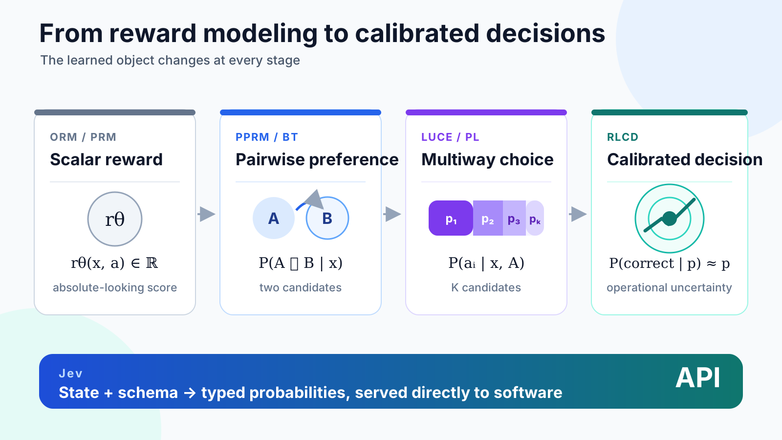
Jev looks mysterious when viewed as an alternative to a language model. It becomes much simpler when viewed as the next step in reward modeling.

The core idea is:

\[ \text{RLCD} = \text{multiway preference modeling} + \text{probability calibration} \]

More specifically, RLCD is a schema-conditioned Plackett–Luce objective. Jev turns that objective into a product by adding typed outputs and parallel inference.

That is the secret: the reward model is no longer hidden behind a generator. The reward model becomes the model.

Reward Modeling Started with a Scalar

A conventional reward model receives a context \(x\) and a candidate answer \(a\), then produces a scalar:

\[ r_\theta(x,a)\in\mathbb{R} \]

Outcome reward models score the final answer. Process reward models score individual reasoning steps. In both cases, the learned object is an absolute-looking number.

The problem is that this number is not actually absolute.

A reward of \(0.8\) does not have a stable meaning across problems, candidate pools, checkpoints, or model families. It is mainly useful for comparing candidates generated under similar conditions:

\[ r_\theta(x,a_1) > r_\theta(x,a_2) \]

The operational signal was always relative preference. The scalar merely hid it.

PPRM Made the Preference Explicit

LLaMA-Berry’s Pairwise Preference Reward Model, or PPRM, exposes the comparison directly.

Given a problem \(x\) and two solutions \(a_1\) and \(a_2\), PPRM answers:

Is the first answer better than the second answer?

Its probability has the form:

\[ P(a_1 \succ a_2\mid x) = \frac{\exp u_\theta(x,a_1)} {\exp u_\theta(x,a_1)+\exp u_\theta(x,a_2)} \]

Equivalently:

\[ P(a_1 \succ a_2\mid x) = \sigma\left( u_\theta(x,a_1)-u_\theta(x,a_2) \right) \]

This is the Bradley–Terry model.

LLaMA-Berry implements the comparison as a constrained language-model decision over Yes and No tokens. It trains the evaluator on almost 7.8 million mathematical-solution pairs and uses DPO to improve the pairwise prediction task. The essential change is conceptual: reward modeling becomes preference-probability modeling. See the LLaMA-Berry paper.

PPRM still contains a latent scalar utility \(u_\theta(x,a)\), but that utility is no longer presented as an absolute reward. It becomes meaningful through a normalized comparison.

LLaMA-Berry subsequently uses Enhanced Borda Count to aggregate pairwise comparisons inside MCTS. That is downstream search machinery. EBC neither defines PPRM’s preference loss nor provides the bridge from PPRM to RLCD.

The relevant lineage is simply:

\[ \text{scalar reward} \rightarrow \text{pairwise preference} \rightarrow \text{multiway preference} \rightarrow \text{calibrated decision} \]

Plackett–Luce Is the Multiway PPRM

PPRM compares two candidates. A real decision interface usually receives more than two.

Let the candidate set be:

\[ A=\{a_1,a_2,\dots,a_K\} \]

Assign each candidate a context-dependent utility:

\[ u_i=u_\theta(x,a_i) \]

Then normalize all candidates together:

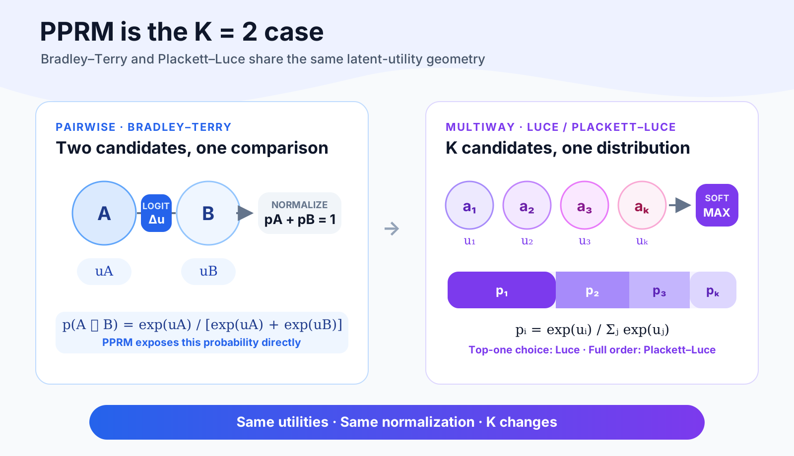
\[ P(a_i\mid x,A) = \frac{\exp u_i} {\sum_{j=1}^{K}\exp u_j} \]

This is the Luce choice model, also known as multinomial logit. It is the top-one form of the Plackett–Luce family.

When \(K=2\), it reduces exactly to Bradley–Terry:

\[ P(a_1\mid x,\{a_1,a_2\}) = \frac{\exp u_1}{\exp u_1+\exp u_2} \]

PPRM is therefore the binary case of the same choice geometry.

If the supervision contains a complete ranking

\[ a_{\pi_1}\succ a_{\pi_2}\succ\dots\succ a_{\pi_K}, \]

the full Plackett–Luce likelihood repeatedly selects the next-best remaining candidate:

\[ P(\pi\mid x) = \prod_{t=1}^{K} \frac{\exp u_{\pi_t}} {\sum_{j=t}^{K}\exp u_{\pi_j}} \]

The corresponding loss is:

\[ \mathcal{L}_{\mathrm{PL}} = -\sum_{t=1}^{K} \log \frac{\exp u_{\pi_t}} {\sum_{j=t}^{K}\exp u_{\pi_j}} \]

When the label specifies only one correct choice \(y\), the loss becomes:

\[ \mathcal{L}_{\mathrm{choice}} = -\log \frac{\exp u_y} {\sum_j\exp u_j} \]

That is the first stage of the Plackett–Luce likelihood: a multiway extension of PPRM.

This is the mathematical center of RLCD.

RLCD Adds Calibration

Plackett–Luce gives us a probability distribution, but normalization is not calibration.

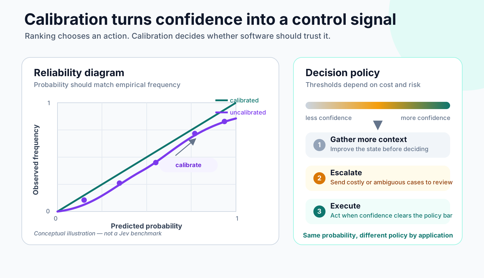
A softmax vector always sums to one. That does not mean a prediction reported as \(0.8\) is correct 80% of the time.

Calibration adds that empirical meaning:

\[ P(Y=\hat{Y}\mid \hat{P}=p)\approx p \]

Across predictions assigned probability \(0.8\), approximately 80% should be correct. This is also the contract TypeSafe gives for RLCD: Jev returns decisions and probabilities, and higher reported probabilities should correspond to higher observed accuracy. See TypeSafe’s RLCD primer.

A minimal implementation uses a proper scoring rule such as log loss:

\[ \mathcal{L}_{\mathrm{NLL}}=-\log p_y \]

Brier calibration: confidence gets a price

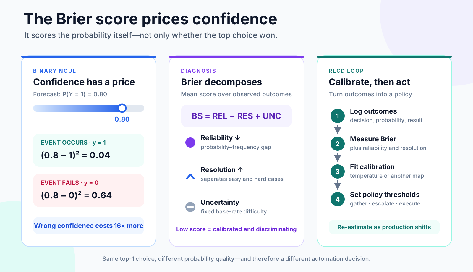
The Brier score makes the calibration objective concrete. For a binary Noul decision, let \(p=P(Y=1\mid x)\) and \(y\in\{0,1\}\). The score is:

\[ \operatorname{BS}(p,y)=(p-y)^2 \]

If the model reports \(p=0.8\), it receives a score of \(0.04\) when the event occurs and \(0.64\) when it does not. The confidently wrong forecast costs sixteen times as much as the confidently correct one.

This is why the Brier score fits a decision model. It is a strictly proper scoring rule: in expectation, the model minimizes the score by reporting the true conditional probability instead of gaming the threshold. The score was introduced for probabilistic forecasts by Glenn Brier; its role as a proper scoring rule is developed by Gneiting and Raftery.

For a multiway Choice, the score extends to the full probability vector. Using the normalization that makes the two-class case match the binary formula:

\[ \operatorname{BS}(\mathbf{p},y) = \frac{1}{2} \sum_{i=1}^{K} \left(p_i-\mathbb{1}[i=y]\right)^2 \]

This matters because top-1 accuracy discards probability quality. Two models can choose the same action while reporting \(0.55\) and \(0.99\). Once outcomes arrive, Brier score tells us whether that extra confidence was earned.

For binary outcomes, the Murphy decomposition separates the mean score into three terms:

\[ \operatorname{BS} = \operatorname{REL} - \operatorname{RES} + \operatorname{UNC} \]

• Reliability \(\operatorname{REL}\) measures the gap between reported probabilities and observed frequencies. Lower is better.
• Resolution \(\operatorname{RES}\) measures whether the model separates cases with different outcome rates. Higher is better.
• Uncertainty \(\operatorname{UNC}\) is the base-rate difficulty of the evaluation set. It is fixed when models are compared on the same data.

A lower Brier score can therefore come from better calibration, better separation of easy and hard cases, or both. A constant base-rate predictor can be calibrated while having zero resolution; Brier exposes that weakness.

An RLCD implementation can apply Brier score to the decision probabilities during training and use it again as a held-out objective for post-hoc calibration. With temperature scaling, the calibration parameter can be selected directly on validation outcomes:

\[ T^* = \arg\min_{T>0} \sum_{n=1}^{N} \operatorname{BS}\!\left(\mathbf{p}^{(T)}(x_n),y_n\right) \]

Temperature scaling then adjusts the sharpness of the distribution:

\[ p_i = \frac{\exp(u_i/T)} {\sum_j\exp(u_j/T)} \]

Here \(T\) controls how concentrated the probabilities are without changing their ordering. Brier is the objective; temperature scaling is the calibrator. One measures probability quality, while the other changes the distribution.

This separates two objectives that ordinary reward modeling often conflates:

• Ranking asks whether the best candidate appears first.
• Calibration asks whether the model knows how often that decision is right.

Automation needs both. Ranking selects an action; calibration determines whether software should execute it, defer it, or escalate it.

The useful abstraction is:

\[ \text{RLCD} = \text{Plackett–Luce preference loss} + \text{calibration constraint} \]

Jev Turns the Reward Model into the Product

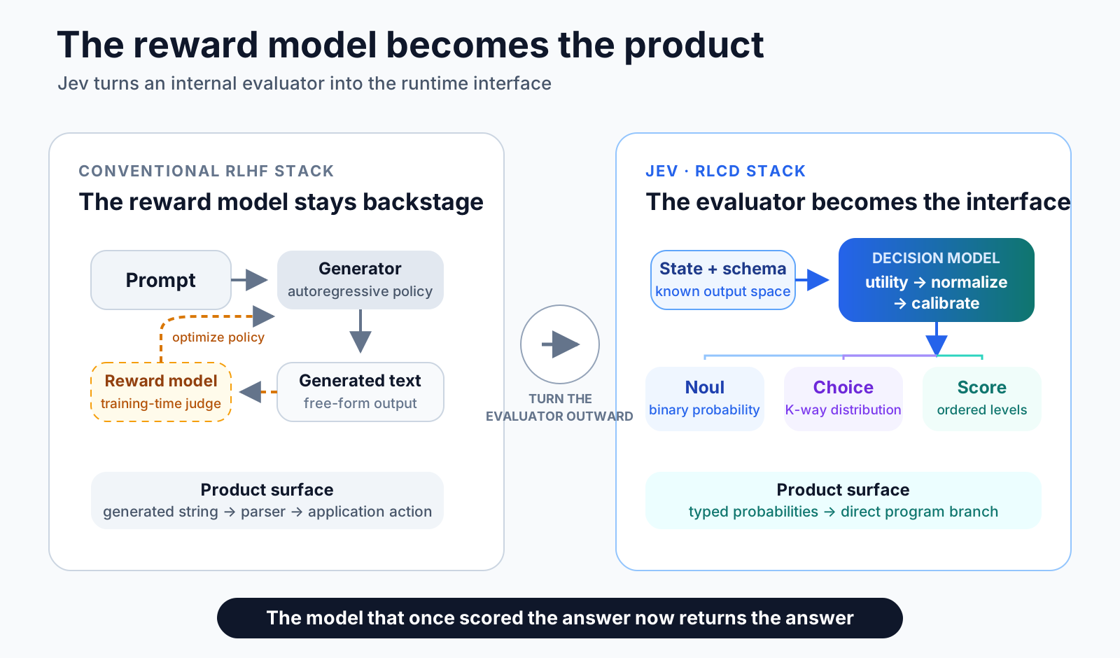
In the conventional RLHF stack, the reward model is an internal component:

\[ \text{prompt} \rightarrow \text{generator} \rightarrow \text{candidate response} \rightarrow \text{reward model} \]

Users interact with the generator. The reward model only trains or evaluates it.

Jev reverses that architecture:

\[ \text{state} + \text{candidate schema} \rightarrow \text{calibrated decision distribution} \]

There is no need to generate an explanation and parse it back into an action. The evaluator itself becomes the runtime interface.

Jev exposes three primitives:

Jev primitive	Preference-model interpretation
Noul	Binary Bradley–Terry decision between true and false
Choice	Luce distribution over \(K\) unordered alternatives
Score	Distribution over an ordered set of levels

A Choice returns the selected option, the complete probability distribution, and a confidence value. A Score returns a position along user-defined levels together with the distribution across those levels. A Noul returns the probability that a proposition is true. See Jev’s primitive documentation.

These are not three unrelated capabilities. They are three schemas over the same underlying object:

\[ P(\text{typed outcome}\mid \text{state},\text{question},\text{candidate set}) \]

Jev is therefore a reward model generalized from “Which answer is better?” to “Which typed outcome should the program select?”

The Decision Head Produces the Utilities

The Plackett–Luce equations leave the utility \(u_\theta(x,a_i)\) abstract. The decision head is the component that computes it.

In Jevre, the encoder processes the state, question, and every candidate under the tree attention mask. The model mean-pools the normalized hidden states of the three spans:

\[ \bar{h}_S, \qquad \bar{h}_{Q_f}, \qquad \bar{h}_{C_{f,i}} \]

For question \(f\), the state and question form a query. Each candidate forms a key:

\[ q_f = W_q\bar{h}_S + W_q\bar{h}_{Q_f}, \qquad k_{f,i} = W_k\bar{h}_{C_{f,i}} \]

The candidate utility is their scaled inner product:

\[ u_{f,i} = \frac{q_f^\top k_{f,i}}{\sqrt{r}} \]

The released model uses \(r=512\). This rank is the dimension of the learned interaction space; the encoder and decision head are trained together. A softmax across the candidates of the same question turns the utilities into the RLCD distribution:

\[ p_{f,i} = \frac{\exp u_{f,i}} {\sum_j \exp u_{f,j}} \]

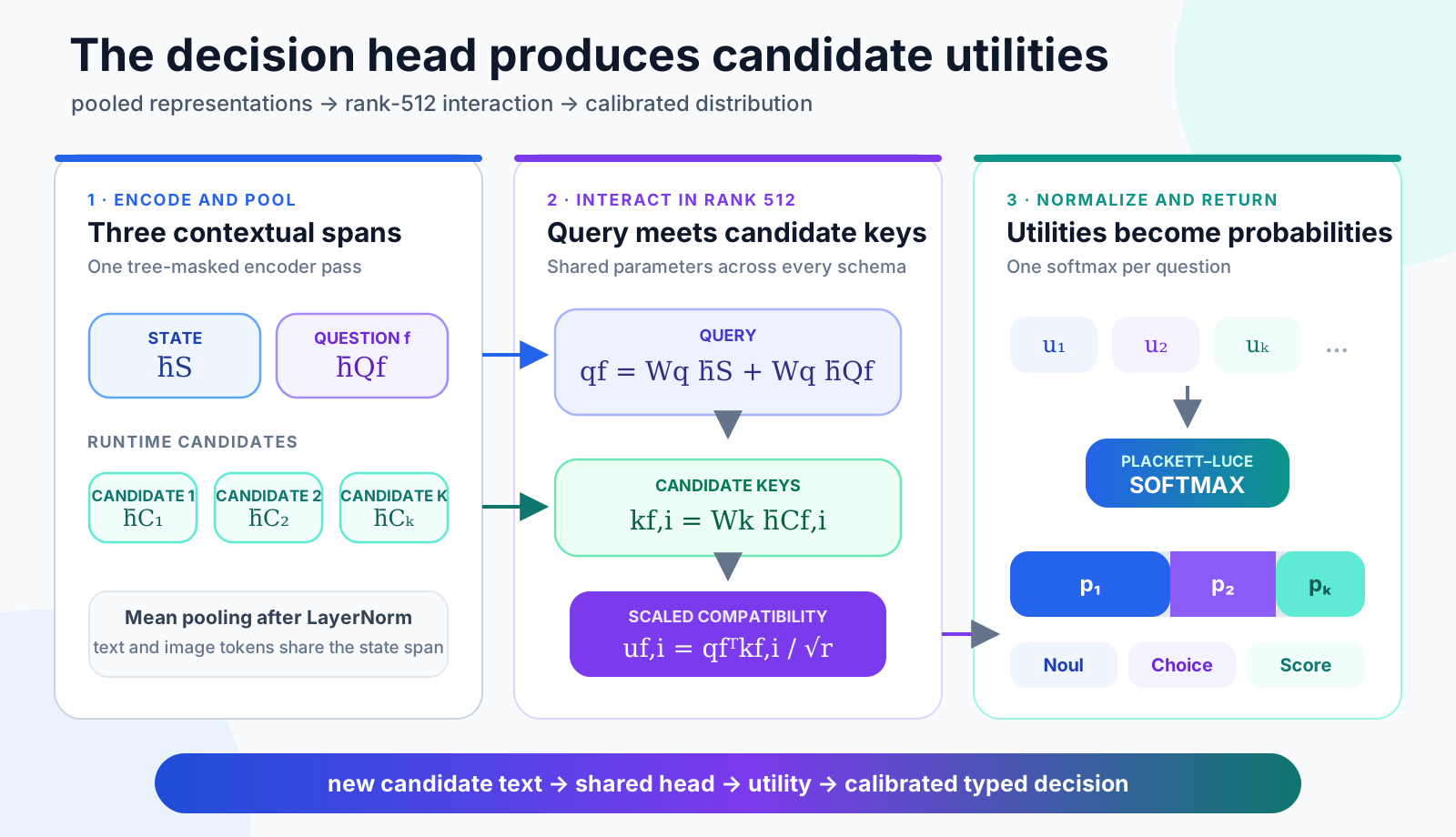
This head scores contextual representations rather than vocabulary labels. Candidate names and descriptions arrive at runtime as text, so the same parameters can score a new schema without adding a class-specific output layer. Noul, Choice, and Score all use these logits; the schema decoder determines how the resulting distribution is returned.

Images enter through the state span and change \(\bar{h}_S\), while the decision head stays unchanged. The same utility function therefore covers text and multimodal decisions. The full implementation is visible in the scorer model and the released Jevre checkpoint.

The decision head is the bridge between representation learning and RLCD: the encoder builds state-, question-, and candidate-aware representations; the head turns their compatibility into utilities; Plackett–Luce and Brier training shape those utilities into calibrated decisions.

Why Jev Can Run in Parallel

Strip away the branding: Jev’s parallel sampler is sequence packing plus an attention mask, followed by one shared decision head and typed schema decoding. This is the serving trick behind the speed claim.

Autoregressive language models represent an answer as a token sequence:

\[ P(y\mid x) = \prod_{t=1}^{T} P(y_t\mid x,y_{<t}) \]

Every token depends on the previous tokens. Latency grows with output length.

A decision model already knows its output space. It only needs to estimate utilities and normalize them:

\[ x,A \rightarrow (u_1,\dots,u_K) \rightarrow (p_1,\dots,p_K) \]

No sentence has to be decoded.

Now pack the shared state, questions, and candidate branches into one sequence:

\[ Z = [S;Q_1;C_{1,1};\dots;C_{1,K_1};Q_2;C_{2,1};\dots;C_{m,K_m}] \]

The packed sequence is only the physical layout. Its logical layout is a tree:

\[ S \rightarrow Q_q \rightarrow C_{q,k} \]

The attention mask preserves that tree. A question reads the shared state and itself. A candidate reads the shared state, its own question, and its own candidate tokens. It cannot read another question or a sibling candidate. Let \(v(i)\) denote the tree node containing token \(i\), and let \(v(j)\preceq v(i)\) mean that \(v(j)\) is an ancestor of, or identical to, \(v(i)\). Then:

\[ M^{\mathrm{tree}}_{ij} = \begin{cases} 0, & v(j)\preceq v(i),\\ -\infty, & \text{otherwise}. \end{cases} \]

For a causal backbone, this structural mask is combined with causal order inside each branch. Position IDs reset at every branch: all questions start after the same state prefix, and all candidates under a question start after the same state-plus-question prefix. Candidate \(C_{q,2}\) therefore gains no information merely because it was packed after \(C_{q,1}\).

\[ \operatorname{Attn}(Q,K,V;M) = \operatorname{softmax}\!\left(\frac{QK^{\top}}{\sqrt d}+M\right)V \]

The result is one accelerator-friendly forward pass that produces every candidate score together. Packing removes repeated prefixes. Tree attention prevents cross-question and cross-candidate contamination. The decision head produces utilities, and the schema decoder returns them as Noul, Choice, or Score probabilities. There is no token-by-token generation loop.

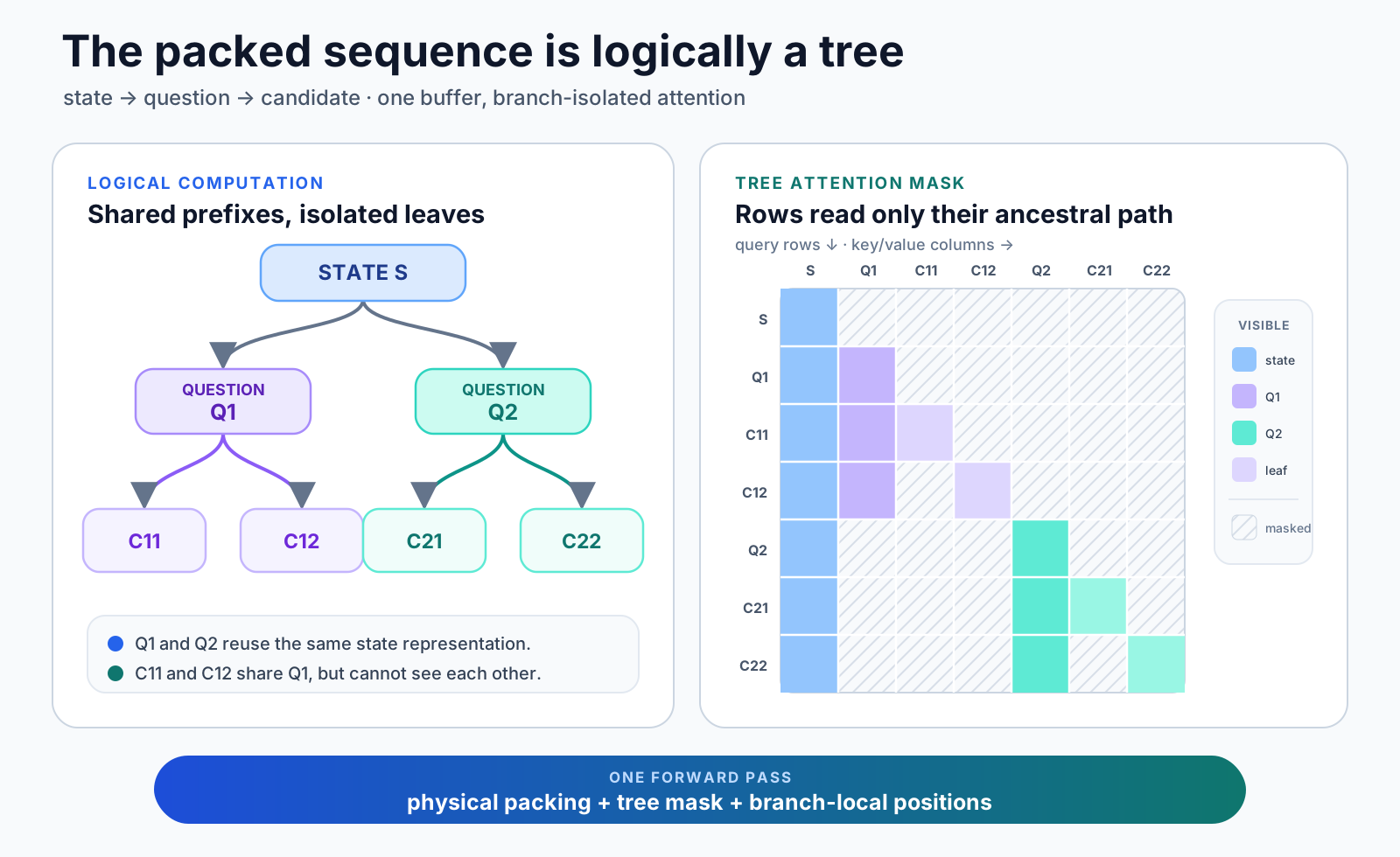
This behavior is exactly the contract in TypeSafe’s documentation: questions share the same state, are evaluated independently, and return in parallel. The mechanism itself is established Transformer engineering. Sequence packing with attention masks that prevent cross-contamination was already documented as a general throughput technique in the sequence-packing literature.

TypeSafe’s launch post names a “new model architecture” and a “parallel sampler,” but it publishes no new attention operator, no sampler algorithm, no complexity result, and no ablation that isolates a novel sampling mechanism. A real sampling breakthrough would make those artifacts the center of the announcement. They are absent. What remains is a productized composition of familiar primitives:

\[ \text{parallel sampler} = \text{packing} + \text{attention mask} + \text{decision head} + \text{schema decoding} \]

For very high-cardinality choices, Jev adds a two-stage procedure: score candidates independently, then make an explicit choice. That is another scheduling decomposition, not a new sampling law. See TypeSafe’s Jev announcement.

The complete system decomposition is therefore:

\[ \text{Jev} = \text{RLCD} + \text{decision head} + \text{typed schemas} + \text{packing} + \text{attention masks} \]

RLCD explains what the model learns. Packing and masking explain how the learned decision function is served efficiently. The engineering is useful. It is not a new class of sampler.

RLCD Is Not a Third Kind of Reward Source

TypeSafe presents RLHF, RLVR, and RLCD as three post-training paths. They are not three mutually exclusive mathematical categories.

RLHF and RLVR primarily describe where the reward comes from:

• RLHF: human preference.
• RLVR: programmatically verifiable outcomes.

RLCD describes what the model is trained to return:

• a constrained decision;
• a probability distribution;
• calibrated uncertainty.

Human comparisons can train RLCD. Verifiable outcomes can train RLCD. Synthetic judges can train RLCD. Logged production outcomes can train RLCD.

The word reinforcement learning describes the broader post-training pipeline. The statistical heart of the objective is preference estimation under a proper probabilistic loss. PPO is not required to obtain this structure.

The cleaner taxonomy is:

Method	Primary training signal	Product output
RLHF	Human preference	Generated response
RLVR	Verifiable reward	Generated reasoning or answer
RLCD	Decision outcome and calibration	Typed probability distribution

RLCD is defined by the output contract, not by a unique source of reward.

The Thesis Produces Testable Predictions

If Jev is a calibrated, schema-conditioned Plackett–Luce model, its behavior should expose several measurable properties.

1. Binary equivalence

A two-option Choice and an equivalent Noul question should produce closely aligned probabilities:

\[ P(A\mid\{A,B\}) \approx P(A\succ B) \]

2. Pairwise–multiway consistency

For two candidates inside a larger set:

\[ \frac{P(a_i\mid A)}{P(a_j\mid A)} \approx \exp(u_i-u_j) \]

Their relative odds should match a direct pairwise comparison when the context and wording are held constant.

3. Candidate-set sensitivity

Vanilla Plackett–Luce satisfies independence of irrelevant alternatives. Adding an unrelated candidate should preserve the odds between existing candidates:

\[ \frac{P(a_i\mid A)}{P(a_j\mid A)} = \frac{P(a_i\mid A\cup\{a_k\})} {P(a_j\mid A\cup\{a_k\})} \]

Violations measure how strongly Jev’s utility encoder jointly represents the candidate set.

4. Empirical calibration

Predictions can be placed into probability bins. For the \(0.8\) bin, observed accuracy should approach \(0.8\). For Noul, report the reliability curve, mean Brier score, and Murphy decomposition together. For Choice, report multiclass Brier score and classwise reliability. These views distinguish a useful calibrated model from one that stays safe by predicting the base rate for every case.

5. Order symmetry

Permuting the order of candidate definitions should permute the returned probabilities without changing their values. Any systematic position effect reveals schema-order bias.

These tests turn the RLCD interpretation into a falsifiable model of Jev’s behavior.

Conclusion

Jev is not fundamentally a language model that learned to emit cleaner JSON. It is a preference model promoted into a software interface.

PPRM provides the first step:

\[ \text{absolute reward} \rightarrow \text{pairwise preference probability} \]

Plackett–Luce provides the multiway extension:

\[ \text{pairwise preference} \rightarrow \text{distribution over candidate actions} \]

Calibration makes that distribution operational:

\[ \text{choice probability} \rightarrow \text{automation threshold} \]

Jev packages the result as typed, parallel inference. Its decision head turns contextual representations into candidate utilities, and RLCD turns those utilities into a calibrated multiway distribution served as an API.

The deepest shift is not from one reinforcement-learning algorithm to another. It is from generating an unconstrained answer to estimating a calibrated distribution over actions already defined by software.

Jev is what happens when the reward model stops grading the product and becomes the product.