How to build a diffusion language model

Introduction: Autoregressive and Diffusion Language Models

Two families of generative AI algorithms are widely used today. For continuous data such as images or video, the state-of-the-art approach is based on diffusion models. For discrete data such as text or code, the standard approach is instead autoregressive models. This article explores an alternative for discrete data, one built on the modern paradigm of diffusion.

Mainstream language models are autoregressive: they generate tokens left-to-right, one at a time, each conditioned on the tokens before it. This approach is powerful, but it also has inherent limitations:

• No error correction: once a token is emitted it cannot be revised, so early mistakes compound.
• Generation is slow: producing a sequence takes as many steps as there are tokens, and does not naturally lend itself to fast, parallel generation.
• Causal attention: generation only ever looks backward, never at future context.

Diffusion models take a different approach. Rather than producing text one token at a time, they generate the whole sequence at once, starting from an initial guess and iteratively refining it over a number of steps. This unlocks several advantages: generation can trade off speed and quality by using fewer or more steps, mistakes can be corrected along the way, and every step attends to bidirectional context.

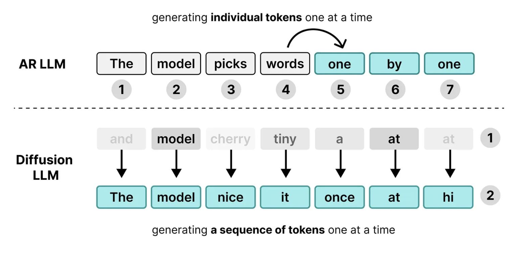
Applying diffusion to language had long been an open problem. In 2024 the field reached a turning point, as diffusion models became competitive with autoregressive models on quality. By 2026, diffusion LLMs are a reality, with releases from leading industry labs — Mercury 2 (Inception Labs) , Gemma Diffusion (Google) , and Nemotron Diffusion (NVIDIA) . This article traces the ideas and papers that underlie these modern models.

Background: Gaussian Diffusion

Before introducing diffusion for language, we start with a brief overview of Gaussian diffusion for image generation. We will then build up discrete diffusion by analogy.

Generating by iterative denoising

The central concept underlying diffusion models is denoising. Instead of painting an image in one shot, a diffusion model produces images step by step, starting from pure random noise and removing a little of it at every step until a coherent image emerges. Generating an image through many small steps turns out to be far simpler than producing it all at once, and this is what makes diffusion models so effective.

How does a model learn to denoise? The trick is to teach it by showing examples of noise being gradually transformed into an image. Diffusion achieves this via two complementary processes. First, a forward process takes a clean source image and turns it into pure noise, one step at a time. Second, a reverse process learns to invert this transformation, turning pure noise back into an image; it is trained on the image-to-noise trajectories produced by the forward process.

Forward process

The forward process takes a clean training image and produces a sequence of increasingly noisy images that trace a path from clean data to pure noise. It does this by mixing in a growing amount of random Gaussian noise at each step, until the image dissolves into pure static. This step requires no learning at all — we are simply adding noise — yet it is enormously useful, because it manufactures an endless supply of training data: examples of images being transformed into noise, and vice versa.

Reverse process

The reverse process is where the actual learning happens. We train a model to transform noise into images by following the steps produced by the forward process in reverse.

Concretely, given a noisy image, we train a machine learning model to separate the noise from the underlying image or, equivalently, to predict either the noise that was added or the clean image itself, since given the noisy input, knowing one determines the other. Once the model can do this, generation is simple: start from pure noise, ask the model to estimate and strip away a bit of it, and repeat. Each pass nudges the sample a little closer to something that looks like real data, until a clean image remains.

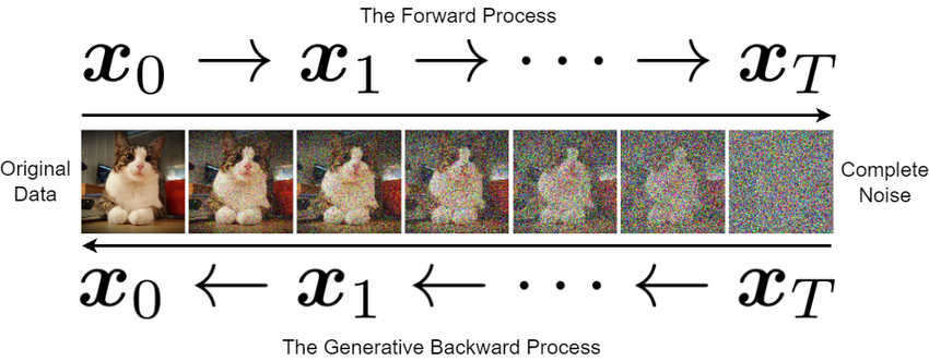
This forward/reverse recipe — corrupt data with noise, then learn to reverse the corruption one step at a time — is the blueprint for every diffusion model.

Simple Masked Diffusion Models

The main obstacle in bringing diffusion to language is deciding what "noise" should mean for discrete tokens. For example, the noise used in classical diffusion is Gaussian, and adding continuous Gaussian noise to categorical variables is not well-defined. Below we introduce one simple yet effective approach that defines noise via masking. Our group popularized this approach, and it now forms the basis of most open-source diffusion language models.

Masked Diffusion in a Nutshell

The easiest way to understand masked diffusion is as an unmasking transformer. We train the model by taking clean sequences, masking a random fraction of their tokens, and asking a bidirectional transformer to fill in the blanks. If you know BERT, this is essentially BERT with a randomized masking rate — but unlike BERT, the resulting model is generative. You can think of masked diffusion as a generative BERT.

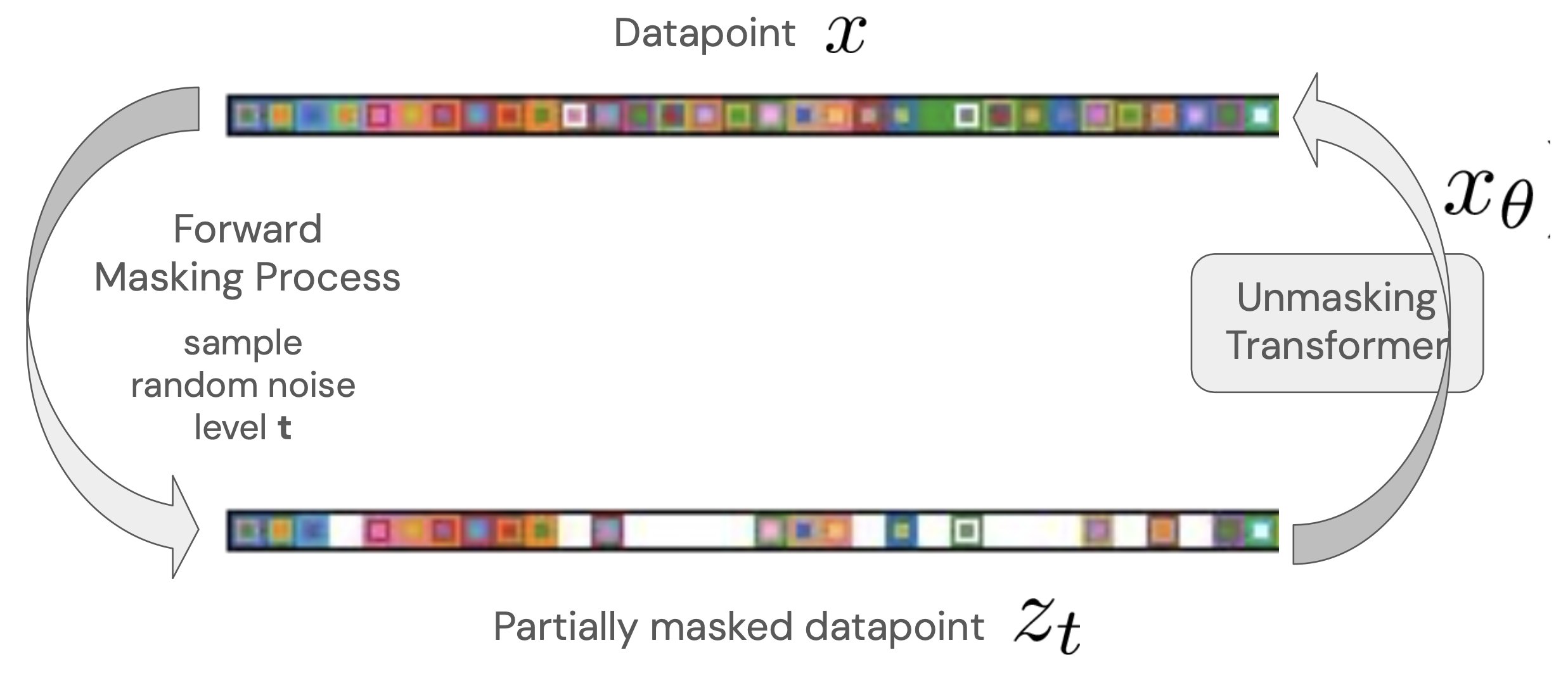
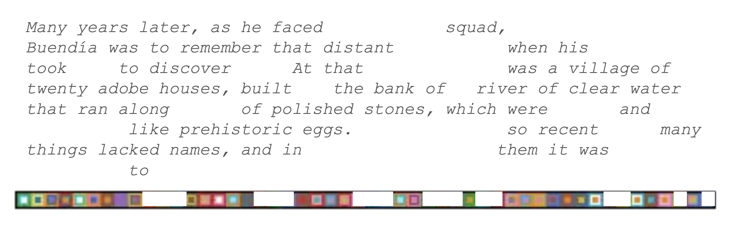
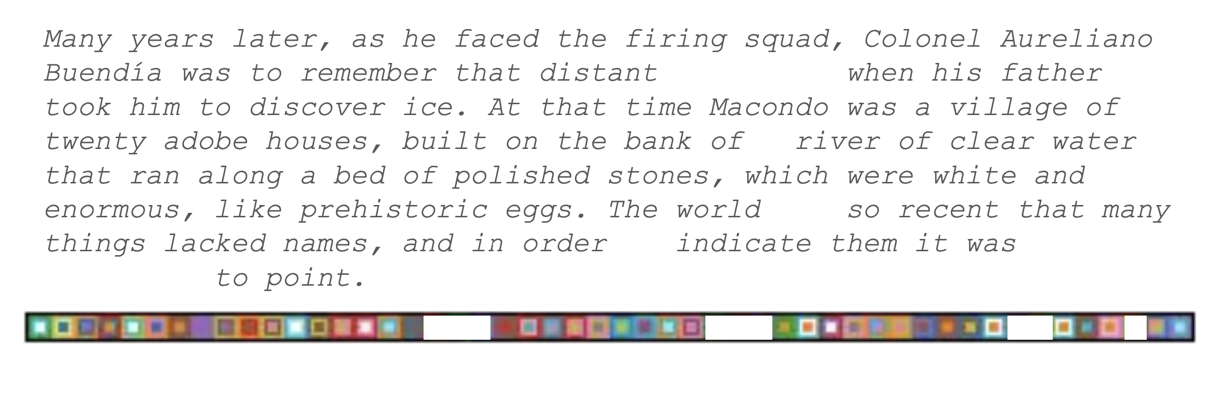
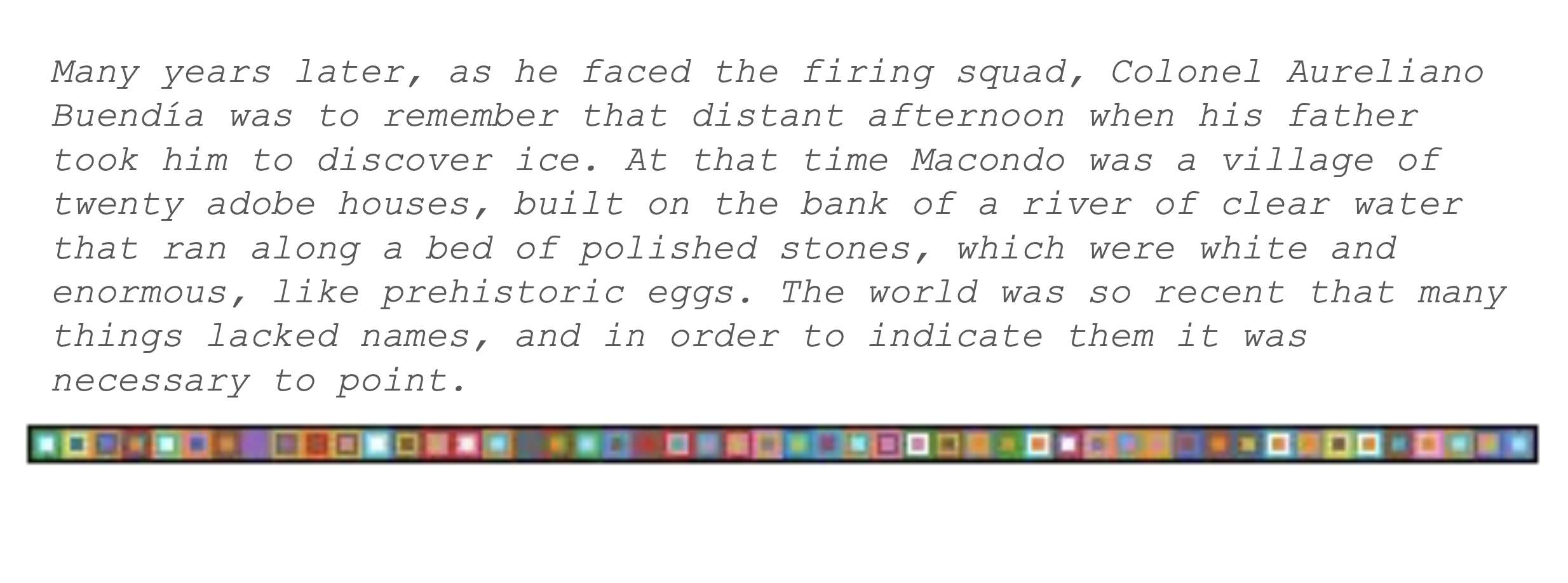
Once we trained the unmasking transformer, we can generate text by starting from a fully masked sequence and repeating two steps many times:

1. Infilling: Ask the model to fill in every blank in the current sequence, yielding a rough guess of the clean tokens.
2. Remasking: Randomly re-noise the infilled sequence by replacing tokens with masks, but keep a few more tokens unmasked than in the previous round.

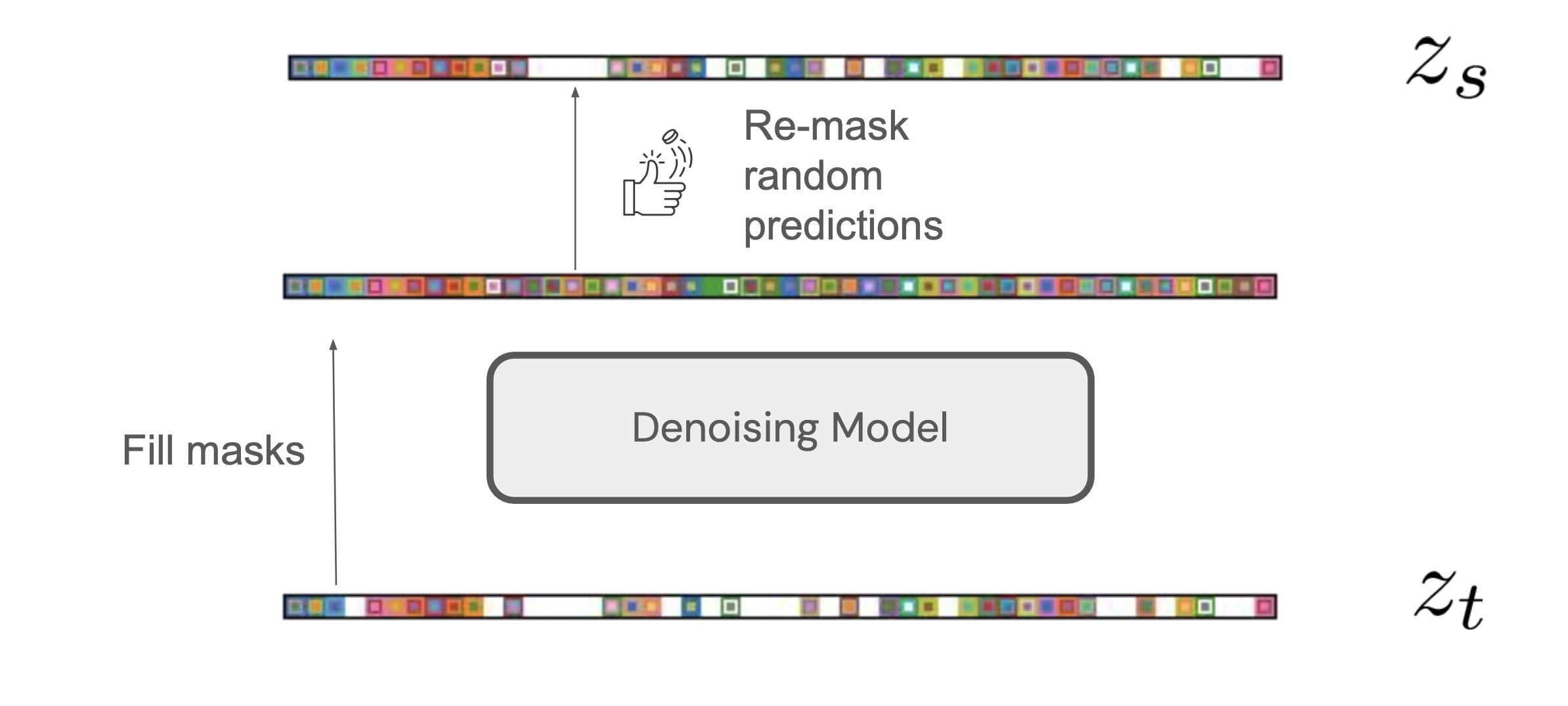
Each round leaves fewer positions masked, until the sequence converges to a clean sample from the model. Generation thus amounts to starting from a sequence full of blanks and gradually filling in words in an arbitrary order.

Understanding Masked Diffusion: A Probabilistic Perspective

We can also understand a bit better why this process works by framing it as an analog of the Gaussian diffusion model we saw earlier. Just like Gaussian diffusion, masked diffusion can be described as a model consisting of a forward and a reverse process.

Forward process

The goal of the forward process is to generate training data for the reverse process. Its output is a trajectory that starts from a datapoint and ends at a sequence of pure noise; the reverse process will then be trained to produce this trajectory in reverse.

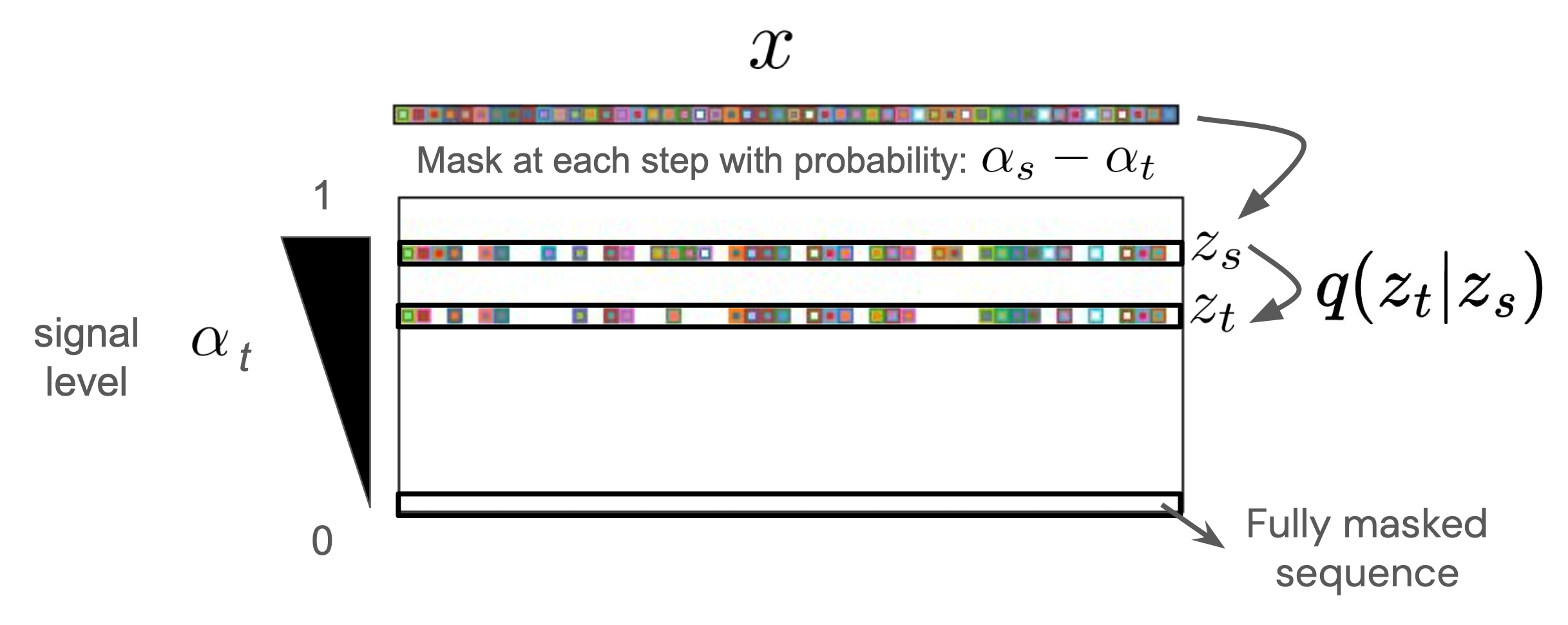
The key challenge is deciding what "noisy" should mean. In Gaussian diffusion, we added varying amounts of white noise to an image. In masked diffusion, we instead randomly mask a fraction of the tokens in a discrete sequence. The amount of masking is governed by a schedule $\alpha_t$ — the probability that a given token remains unmasked — which plays the role of the signal-to-noise ratio in Gaussian diffusion. It starts at $1$ when $t = 0$ (a clean sequence) and decreases to $0$ when $t = 1$ (a fully masked sequence). The time variable $t$ indexes a path from clean to noisy data, and at time $t$ a partially masked sequence $z_t$ has, in expectation, a fraction $\alpha_t$ of its tokens unmasked.

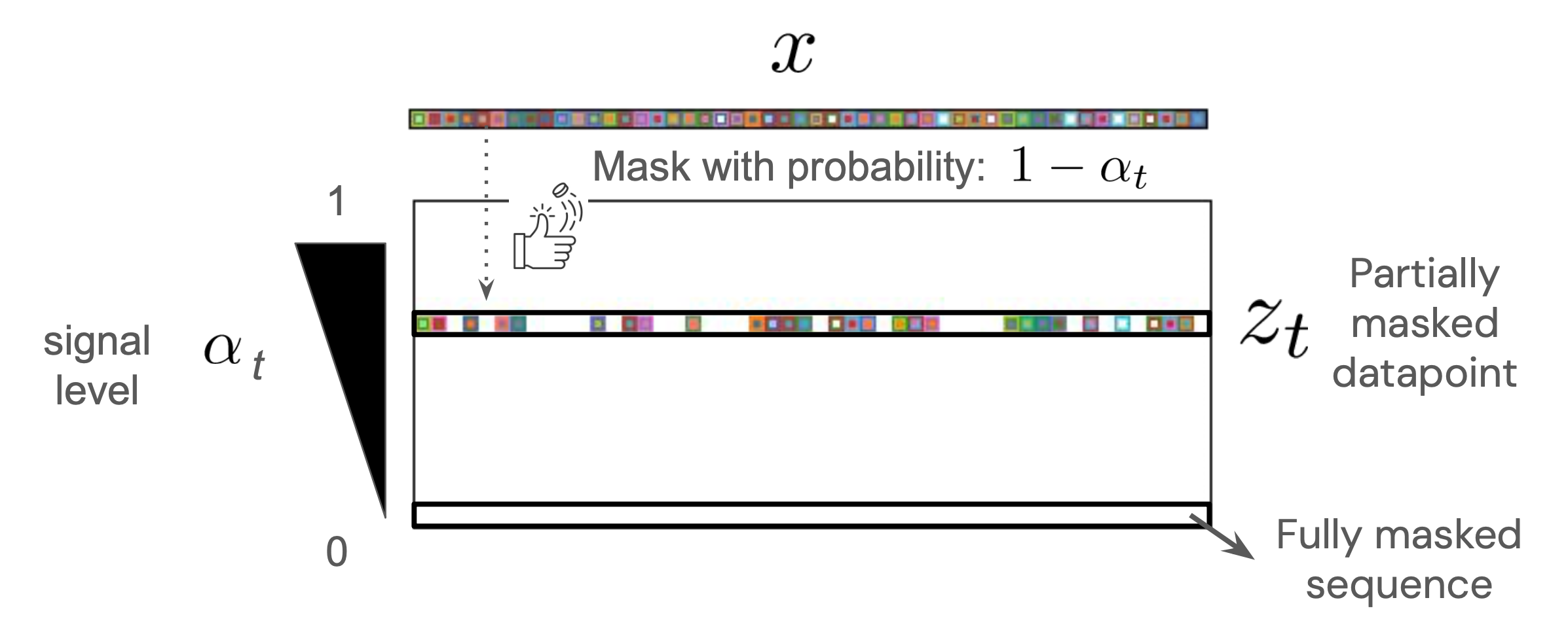
We implement this process as a Markov chain over a sequence of variables $z_t$ indexed by $t$, with $z_0$ being the clean, unmasked sequence. For $s < t$, the chain defines $q(z_t \mid z_s)$ by masking each still-unmasked token of $z_s$ with probability $(\alpha_s - \alpha_t)/\alpha_s$. Running this Markov chain for a number of steps produces a trajectory going from clean data to fully masked noise.

Reverse process

Next, as in Gaussian diffusion, we train the reverse process to walk the sequence of increasingly masked latents in reverse — starting from a fully masked sequence and ultimately generating outputs similar to clean data.

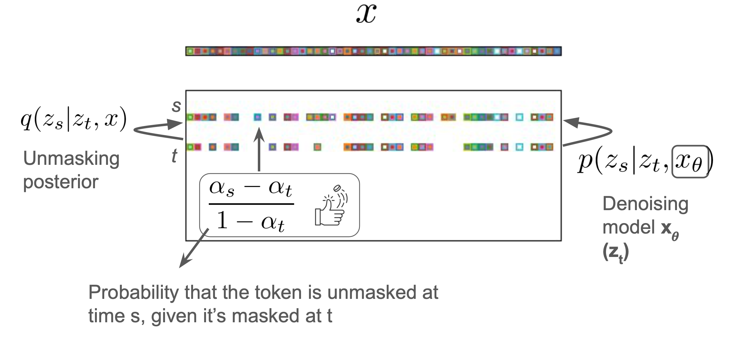
Using Bayes' rule, we can derive the mathematically optimal reverse process $q(z_s \mid z_t, x)$ when the clean sequence $x$ is known . This optimal process has two steps: (1) given a partially masked $z_t$, we peek at $x$ to find the true clean tokens; (2) form $z_s$ by replacing each masked position of $z_t$ with its value in $x$ with probability $(\alpha_s - \alpha_t) / (1 - \alpha_t)$, and otherwise leaving it masked.

In practice, the final output $x$ is obviously unknown when we generate it. We therefore train a model $x_\theta(z_t)$ to predict the final clean sequence given the current state $z_t$ and apply the ideal reverse process $q(z_s \mid z_t, x)$ using the estimate $x_\theta(z_t)$ in place of the real $x$. More formally, we define the reverse process as a probability $p(z_s \mid z_t) = q\big(z_s \mid z_t, x_\theta(z_t)\big)$. This definition recovers the sampling algorithm we described earlier: at each step, we use the model $x_\theta(z_t)$ to fill in the blanks of $z_t$, and we keep a subset of these filled-in tokens in $z_s$.

A probabilistic model for masked diffusion

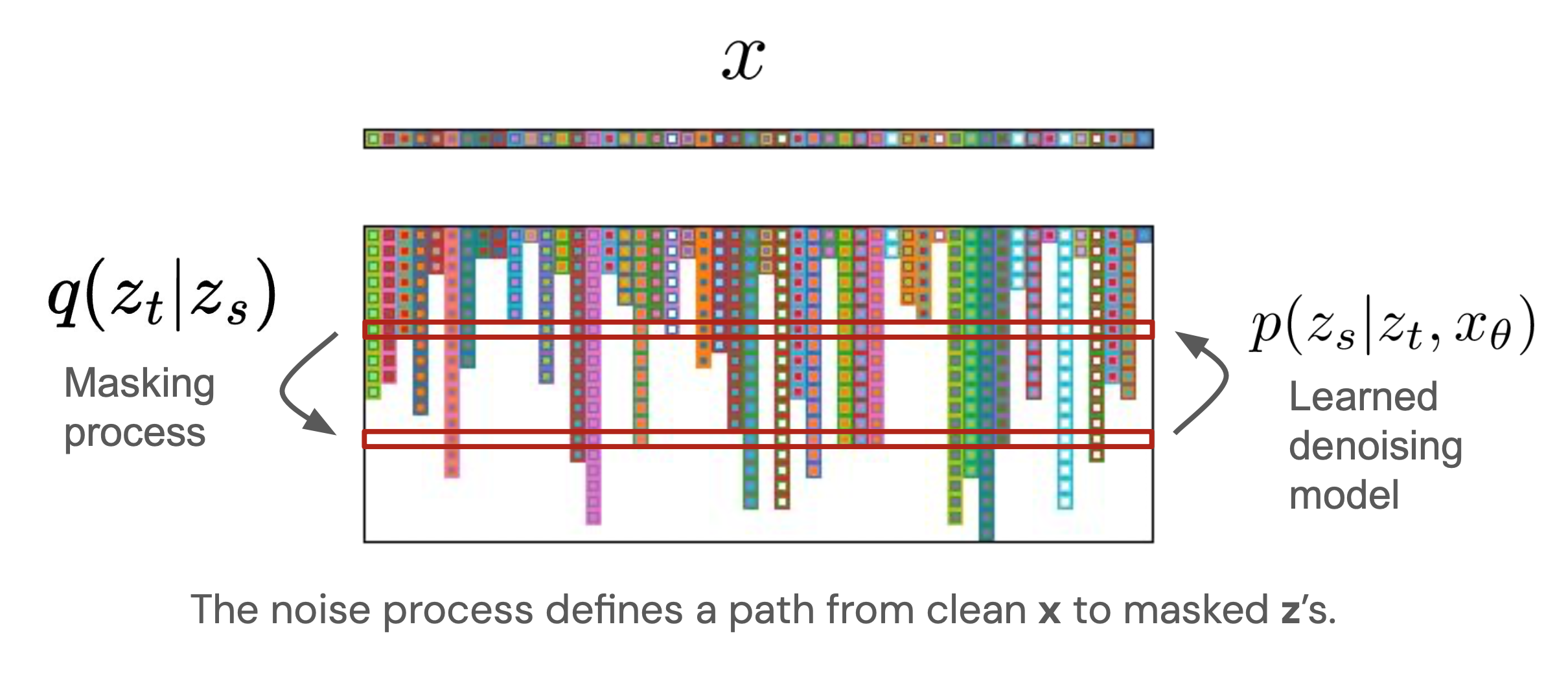
Putting these pieces together gives us the mathematical definition of a masked diffusion language model (MDLM). The forward process $q(z_t \mid z_s)$ produces a trajectory from clean to fully masked data, and the reverse process $p(z_s \mid z_t)$ learns to undo it. Moreover, the reverse process defines a latent variable model $p(x, z_1, \dots, z_T)$ in which $T$ intermediate partially masked samples $z_1,...,z_T$ are latent variables. Generating from the reverse process $p(z_s \mid z_t)$ is the same as performing ancestral sampling from this model.

We can also look at the likelihood $\log p(x)$ of the model $p$ to assess its quality. In latent variable models this is intractable, so we resort to approximations via variational inference. For a masked diffusion language model, the evidence lower bound (ELBO) used to approximate the likelihood has a surprisingly simple form (assuming for simplicity $\alpha_t = 1-t$) :

\[\mathcal{L}_\text{ELBO} = \mathbb{E}_{t \sim \mathcal{U}[0,1]}\; \mathbb{E}_{q(z_t \mid x)} \left[ \frac{1}{t}\, \log p_\theta\!\left(x \mid z_t\right) \right].\]

Let's unpack this formula. The inner term $\log p_\theta(x \mid z_t)$ is the likelihood of a clean sequence $x$ given a partially masked sequence $z_t$ sampled from the forward process. In other words, it is the cross-entropy loss between the predictions of our unmasking transformer and the true tokens — this is exactly the BERT loss!

Differently from BERT, this loss is averaged over all $t$, and hence over all possible masking rates, rather than a single fixed one. It is also normalized by $t$, the expected fraction of tokens that are masked (since $\alpha_t = 1-t$); this factor ensures that each BERT loss is normalized for the number of tokens over which the loss is taken.

Summarizing and Evaluating Masked Diffusion

In summary, MDLM is very similar to BERT, with two key differences:

• It admits principled sampling algorithms, corresponding to ancestral sampling in a latent variable model.
• Training uses a randomized masking rate, which corresponds to a principled variational lower bound on the log-likelihood.

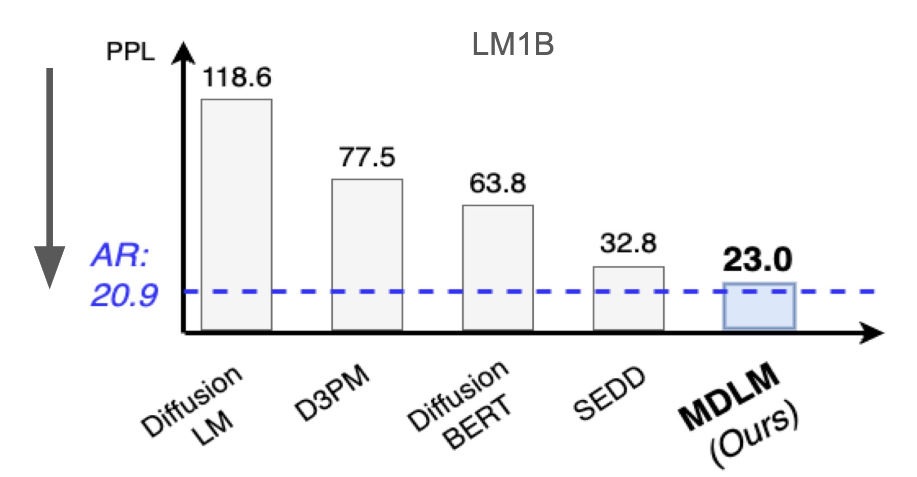
Most interestingly, the evidence lower bound enables a principled comparison between autoregressive and diffusion language models using log-likelihood (or, equivalently, perplexity) — the standard metric for evaluating language models. While for a long time there was a substantial gap in perplexity between diffusion and autoregressive language models, simplified masked diffusion models were among the first to close much of this gap .

Building a Real-World Diffusion Language Model

As defined above, masked diffusion models are helpful for building intuition, but they are not production-ready: they generate only fixed-length sequences, they do not support iterative refinement (error correction) out of the box, and they are not especially fast without additional post-training. The rest of this article explores extensions that address these limitations, in the context of modern open-weights diffusion models.

Block Diffusion for Flexible-Length Generation

The first issue that arises with standard MDLMs is their limitation to generating fixed-length sequences. Block diffusion addresses this limitation by performing diffusion over blocks, conditioned on previously generated tokens . These blocks can be of arbitrary size, ranging from a dozen to thousands of tokens, and should ideally depend on the application domain.

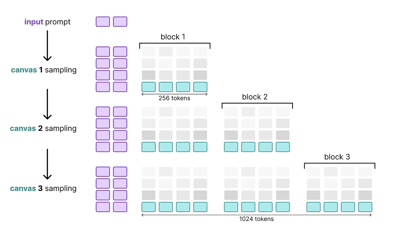
For example, in biological applications, we might have prior knowledge about the length of the interactions we want to capture, and set the block size to the minimum length needed to capture them. In language modeling, we may instead be interested in maximizing GPU utilization; in that case we would choose the block size so that the arithmetic intensity of our forward pass (which also depends on the batch size) matches that of the underlying hardware.

Additionally, block diffusion naturally supports KV caching, a technique that accelerates sequence generation in autoregressive models. Once a block has been generated using a transformer architecture, its keys and values can be cached and reused when generating future blocks.

Other approaches to variable-length generation rely on connections between masked diffusion models and any-order autoregressive models. For instance, Set Diffusion extends block diffusion to operate over arbitrary sets of positions rather than left-to-right blocks. Other approaches, such as Edit Flows or FlexMDM instead model generation as a sequence of insertion, deletion, and substitution operations, which lets the model grow or shrink the sequence as it refines it.

Architectures: Encoder, Decoder, and Encoder–Decoder

Standard masked diffusion models are effectively encoder-only (like BERT), in contrast to decoder-only autoregressive models (like GPT). Using an encoder-only architecture requires sampling algorithms that invoke the full network at every denoising step, which can incur a relatively high computational cost.

A key insight is that diffusion performs two kinds of computation: (1) computing a representation of the tokens that have been generated so far, and (2) denoising the corrupted tokens. This observation suggests using separate modules for each task. The result is an encoder–decoder architecture, which relies on an encoder to represent clean tokens and a lightweight decoder to iteratively refine a noised sequence. Encoder–decoder architectures are at the core of state-of-the-art open-source diffusion LLMs, such as Gemma Diffusion and the recent Nemotron Diffusion models .

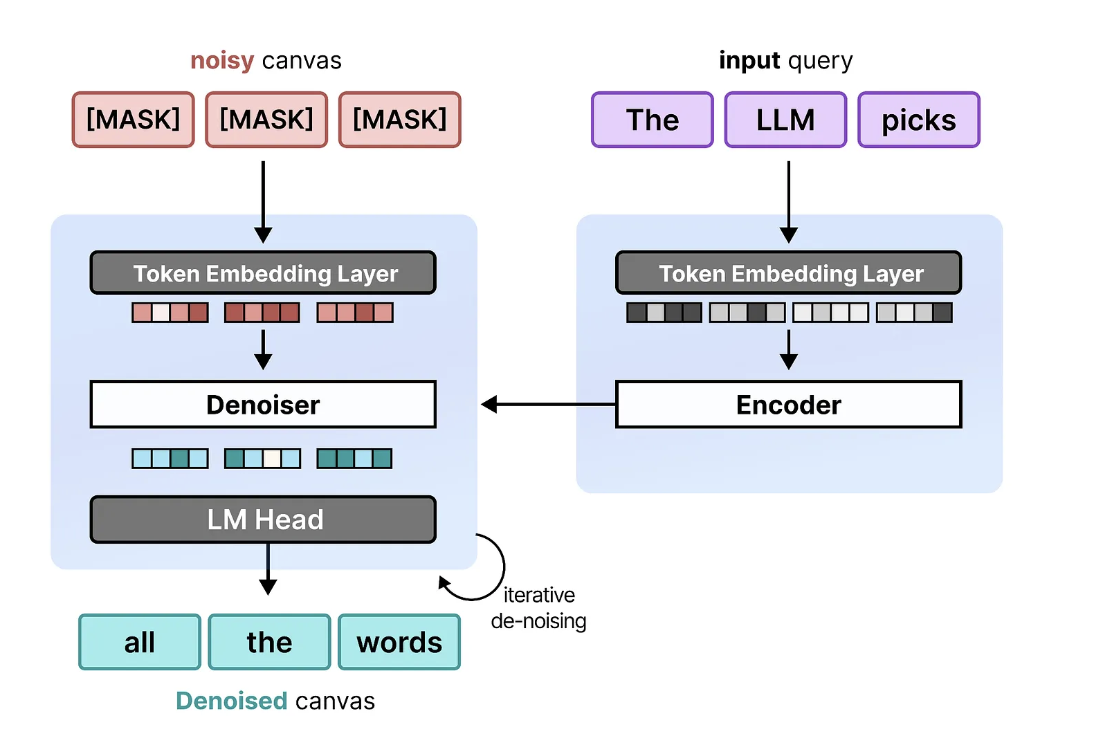
In addition to accelerating discrete diffusion inference, this architecture enables faster training of block diffusion models: after partitioning a sequence into blocks, we pass the blocks into a smaller decoder at training time, which reduces the number of FLOPs needed for training.

Iterative Refinement and Built-In Error Correction

Part of the appeal of diffusion is iterative refinement. Standard MDLMs lack this: once a token is unmasked it can never be updated, because the forward masking process never remasks an unmasked token, so the model never learns to correct itself. Modern diffusion LMs modify the forward and reverse processes to restore this capability.

Remasking Diffusion

The simplest fix is remasking: at each step we keep some newly unmasked tokens but also re-mask a small subset of previously unmasked tokens, letting them be regenerated. Concretely, consider the example below, in which a masked diffusion model introduces a grammatical error. With remasking, this token flips to a mask and then gets corrected when the model receives additional context.

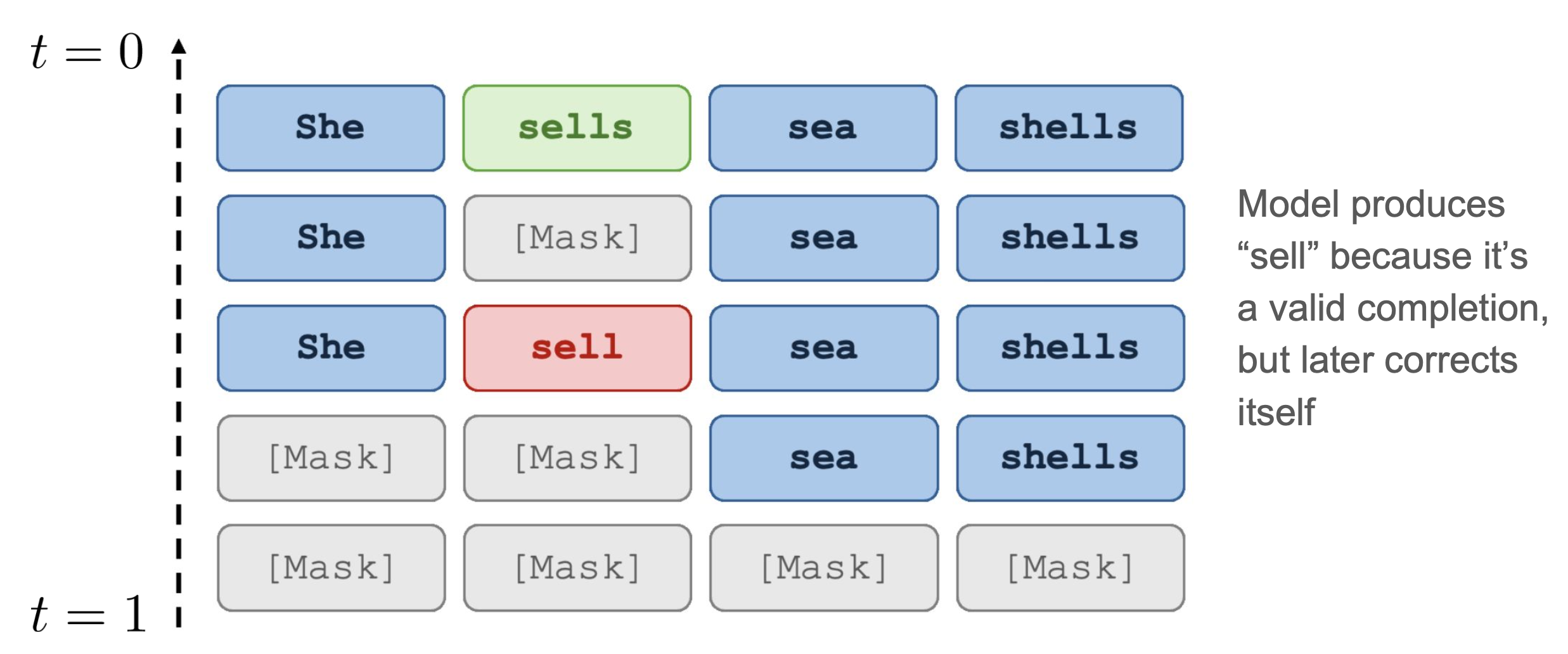
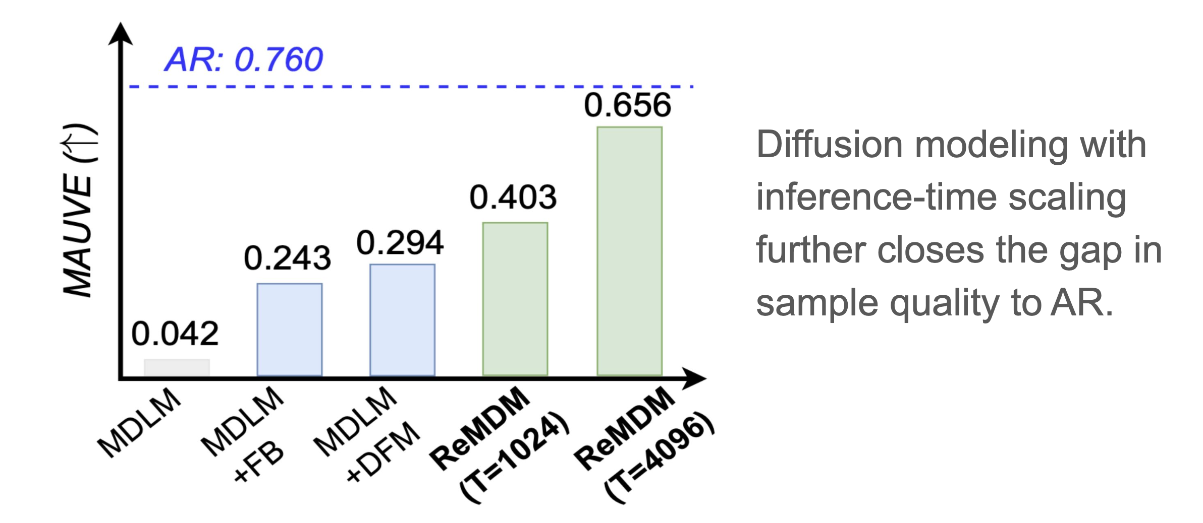
Remasking can be applied to standard pretrained MDLMs in a principled way as a plug-in sampler (formally, it can be seen as implementing a predictor–corrector Markov chain ). Most interestingly, it endows discrete diffusion with a form of inference-time compute scaling: increasing the number of sampling steps lets remasking approach autoregressive quality, while under a tight compute budget it better preserves quality than plain MDLM sampling .

Uniform State Diffusion

Alternatively, we may use an entirely different type of forward and reverse process than masking. Uniform state diffusion is perhaps the most common alternative discrete form of noise. Instead of masking, its forward process replaces tokens with random ones in the vocabulary. The reverse process starts with a random sequence and flips tokens until the result looks like data.

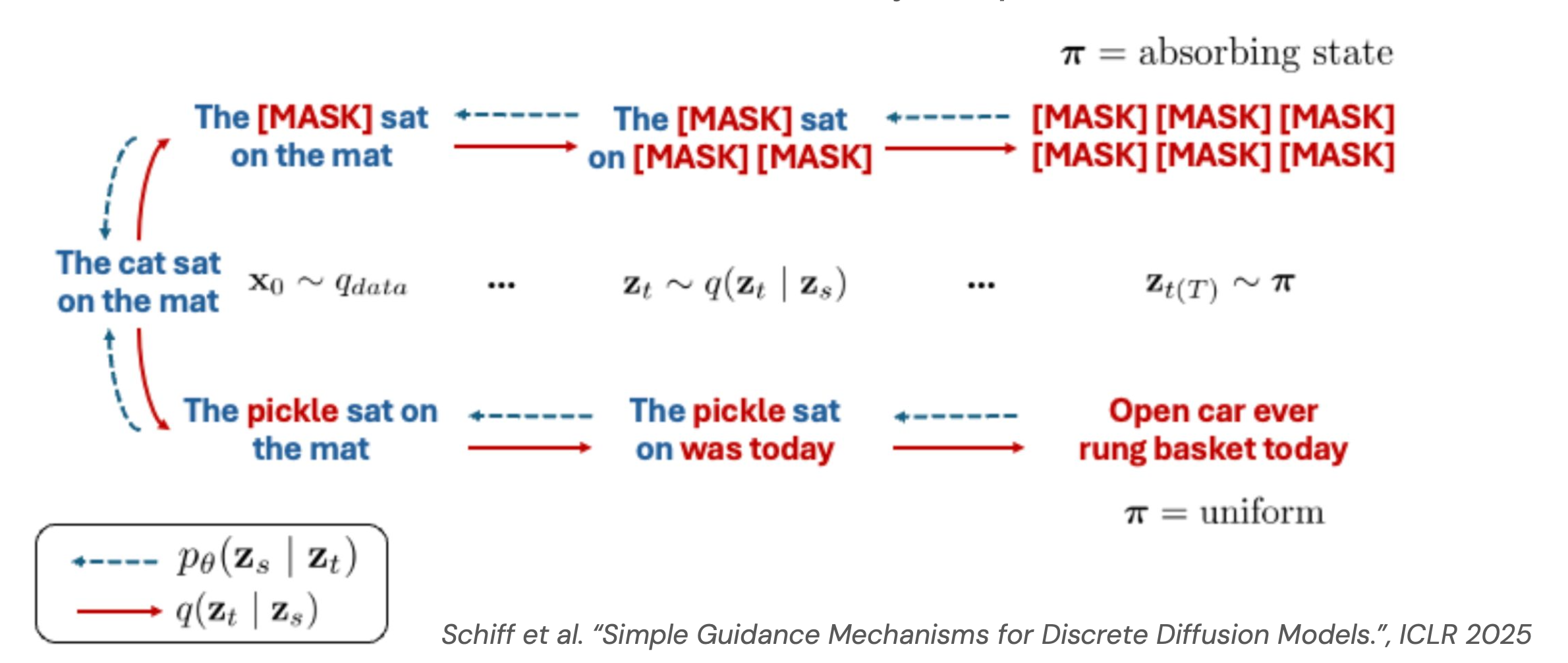
At generation time the model sees a sequence with no masks and decides whether to replace each token, which naturally supports error correction, since any token — not just masked ones — can be revised at any step. While masked diffusion models typically train faster (achieving better perplexities), uniform diffusion language models (UDLMs) facilitate faster sampling and better controllability , as we will discuss below. For instance, the open source Gemma diffusion model is a UDLM.

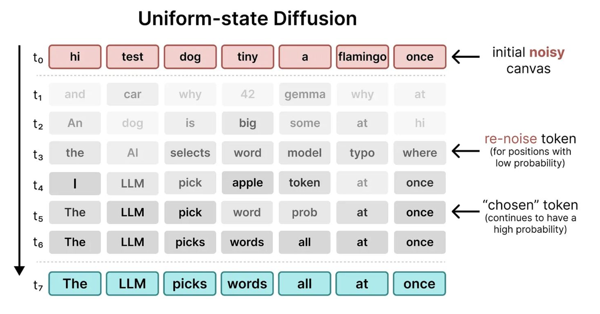
Like MDLM, UDLM supports a simplified evidence lower bound objective that improves training . Earlier, more general frameworks such as D3PM also studied uniform and other structured noise processes, and methods such as generalized interpolating discrete diffusion (GIDD) combine masking and uniform noise into a single process that can recover either as a special case .

Accelerating Diffusion Sampling via Distillation

Because diffusion can generate or refine multiple tokens per step, it can be 5–10× faster than autoregressive generation. However, sampling many tokens at once introduces inconsistencies (e.g., two tokens that disagree in grammatical number, as in the remasking example above); if the underlying noise process cannot correct these errors, they accumulate. This is why most fast diffusion models today rely on error-correcting noise processes such as remasking or UDLM.

Sampling acceleration for these models is often inspired by progressive distillation : a model is trained on its own generations to skip a step, and this is repeated recursively, halving the number of sampling steps each round. In diffusion language models, this idea generalizes to techniques such as self-distillation through time and discrete consistency distillation .

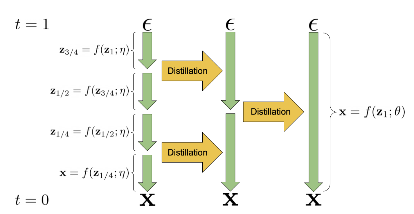
These can be interpreted as a form of on-policy training: standard training is off-policy, since the reverse process is trained on samples from the forward process rather than the samples it will actually see from itself at generation time. Training on the model's own samples in a post-processing step — too expensive to do during primary training — is what enables these methods to improve sampling speed.

Diffusion Enables Controllable Generation

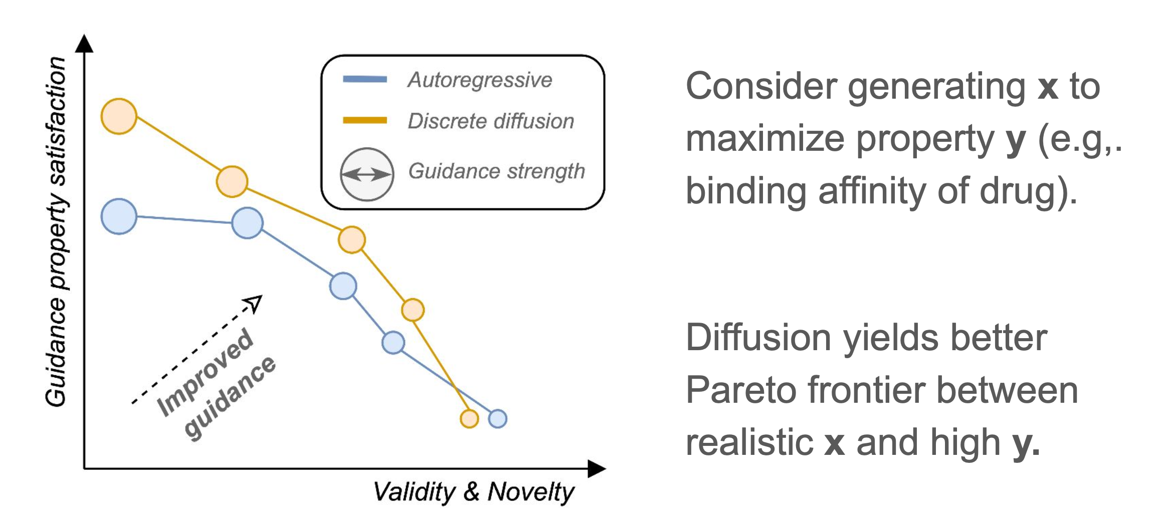
Diffusion models excel at controllable generation: producing a sample $x$ that also satisfies a target property $y$, such as consistency with a prompt if $x$ is an image or binding affinity to a target site if $x$ is a molecule. Because they refine globally rather than committing to irreversible local edits, diffusion models navigate the sample space more effectively and produce better samples with the target property.

In practice, controllability manifests as a Pareto trade-off between naturalness (does the sample look like real data?) and property satisfaction (does it have the property we want?). For example, we could ask the model to produce molecules that look natural, but they might not have the binding affinity we seek. Conversely, we could optimize for binding affinity, but the outputs might not look like natural molecules and not be synthesizable. These two considerations induce a Pareto frontier on which diffusion improves over autoregression.

Algorithms for controllable generation

Diffusion models are especially effective at controllable generation via techniques such as classifier-based guidance (CBG) and classifier-free guidance (CFG). For example, in CBG, if we have a predictor model $p(y \mid x)$ of the target property $y$ given a sample $x$, we can use this model at each step to guide the generation process and provably yield a sample from the conditional distribution $p(x \mid y) \propto p(y \mid x)\, p(x)$.

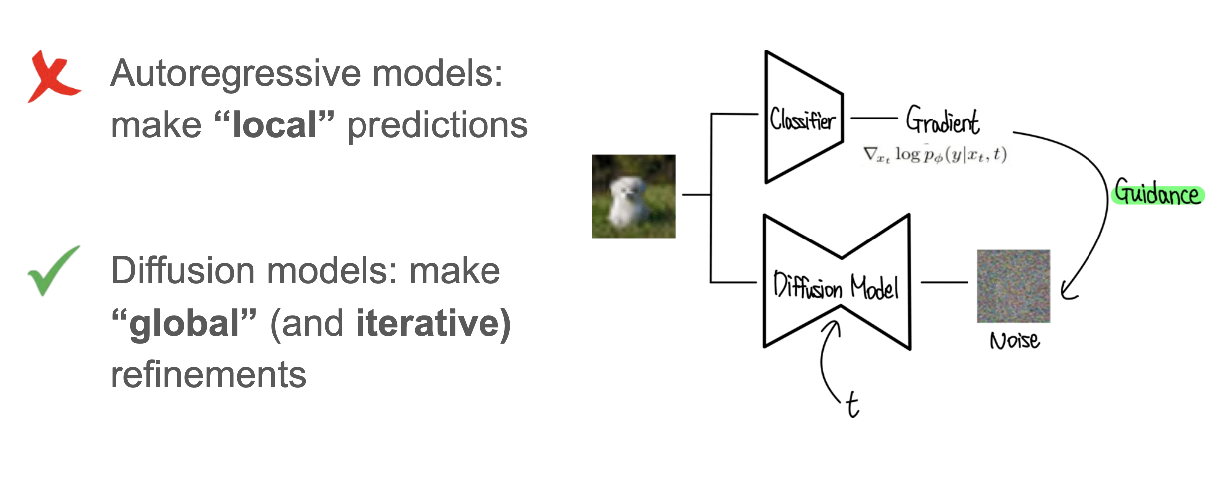
Both techniques extend naturally to MDLM and UDLM , and are especially effective when combined with UDLM or with MDLM plus remasking, since both support revising tokens repeatedly as guidance is applied.

Discrete classifier-based guidance (D-CBG): the math

By Bayes' rule, any conditional reverse process decomposes as follows:

$$ \underbrace{\log p(z_s \mid z_t, y)}_{\text{conditional distribution}} = \underbrace{\log p(y \mid z_t, z_s)}_{\text{predictive term}} + \underbrace{\log p(z_s \mid z_t)}_{\text{unconditional term}} + c, $$

where $c$ is a log-normalization constant. Now suppose we have a classifier $p(y \mid z_t)$ of the property $y$ from a noisy sequence $z_t$, as well as an unconditional diffusion model. We can plug them into the right hand side of the above equation to construct a conditional model from these two individual components.

$$ \underbrace{\log p^{(\gamma)}(z_s \mid z_t, y)}_{\text{new unnormalized distribution}} = \gamma\, \underbrace{\log p(y \mid z_s, z_t)}_{\text{guidance term}} + \underbrace{\log p(z_s \mid z_t)}_{\text{original diffusion model}}, $$

where $\gamma > 0$ is a guidance strength parameter that trades off the property against the model's own preferences. For a single token, the left-hand-side distribution is easy to normalize: we simply sum over the $N$ possible values of that token in the vocabulary. Extending this to a full sequence $z_t^{(1:L)}$ of length $L$ requires additional normalization techniques .

Discrete classifier-free guidance (D-CFG): the math

Instead of training a separate classifier, suppose we have a conditional model $p(z_s \mid z_t, y)$ and an unconditional model $p(z_s \mid z_t)$. Recall the CBG factorization from above,

$$ \log p^{(\gamma)}(z_s \mid z_t, y) = \gamma \cdot \underbrace{\log p(y \mid z_t, z_s)}_{\text{apply Bayes' rule}} + \log p(z_s \mid z_t) + c, $$

and apply Bayes' rule to the classifier term,

$$ \log p(y \mid z_t, z_s) = \log p(z_s \mid z_t, y) - \log p(z_s \mid z_t) + c. $$

Substituting this in and absorbing the $z_s$-independent factors into the normalization constant leaves a simple combination of the conditional and unconditional reverse models:

$$ \underbrace{\log p^{(\gamma)}(z_s \mid z_t, y)}_{\text{new unnormalized distribution}} = \gamma\, \underbrace{\log p(z_s \mid z_t, y)}_{\text{conditional model}} + (1 - \gamma)\, \underbrace{\log p(z_s \mid z_t)}_{\text{unconditional model}}, $$

where $\gamma > 0$ is a guidance strength parameter. This form is convenient because it avoids a separate classifier and, as before, is tractable to normalize: for each token we only sum over its $N$ possible values. In practice, the conditional $p(z_s \mid z_t, y)$ and unconditional $p(z_s \mid z_t)$ distributions are parameterized by the same model, trained by randomly dropping the conditioning signal $y$ so that the network learns both modes at once .

Post-Training Diffusion Language Models

Diffusion language models can also be post-trained with reinforcement learning to improve reasoning, following the same broad recipe that has driven recent gains in autoregressive LLMs. The main complication is that RL algorithms like policy gradient methods need the likelihood of a sampled trajectory, which is easy for autoregressive models (a simple product of next-token probabilities) but expensive for masked diffusion models, whose training objective averages over all masking orders. d1 introduces diffu-GRPO, a critic-free policy-gradient algorithm that estimates these trajectory log-probabilities with a mean-field approximation, combined with masked supervised fine-tuning to distill reasoning behavior from existing datasets . d2 improves on this by deriving more accurate likelihood estimators — an exact one-pass estimator for models that support any-order decoding, and an approximate estimator with a tunable compute–accuracy trade-off otherwise — yielding a new state of the art on logical and math reasoning benchmarks without relying on supervised fine-tuning at all .

Post-training with RL is also central to biological applications of diffusion language models, where the desired reward is often an experimentally measured property (e.g., binding affinity or gene expression) rather than a verifiable answer. Methods such as DRAKES back-propagate this kind of reward through the sampling trajectory of a discrete diffusion model to fine-tune it directly for DNA and protein design , and a broader tutorial surveys the space of RL-based fine-tuning algorithms for diffusion models more generally .

Diffusion Large Language Models Today

Over the last few years, diffusion language models have been scaled up to billions of parameters, showing improvements over autoregressive models at scale. We highlight work in science and language, and we describe how these models are built by combining the basic building blocks introduced above.

Biological and Scientific Domains

One of the first success areas of diffusion language models has been scientific applications, particularly biological sequences. There are two reasons for this:

• Biological sequences are less likely to exhibit the left-to-right biases baked into autoregressive models
• Scientific applications often benefit from controllable generation, which is a natural strength of diffusion

Protein Sequence Modeling

Perhaps the first large scale application of discrete diffusion has been in protein modeling. The recent ESM3 model implements MDLM at up to 100B parameters and is trained on massive amino-acid databases. Both the training and sampling algorithms of ESM3 match the masking diffusion approach described above. The authors report that this approach outperformed autoregressive baselines and set a new state of the art in protein generation.

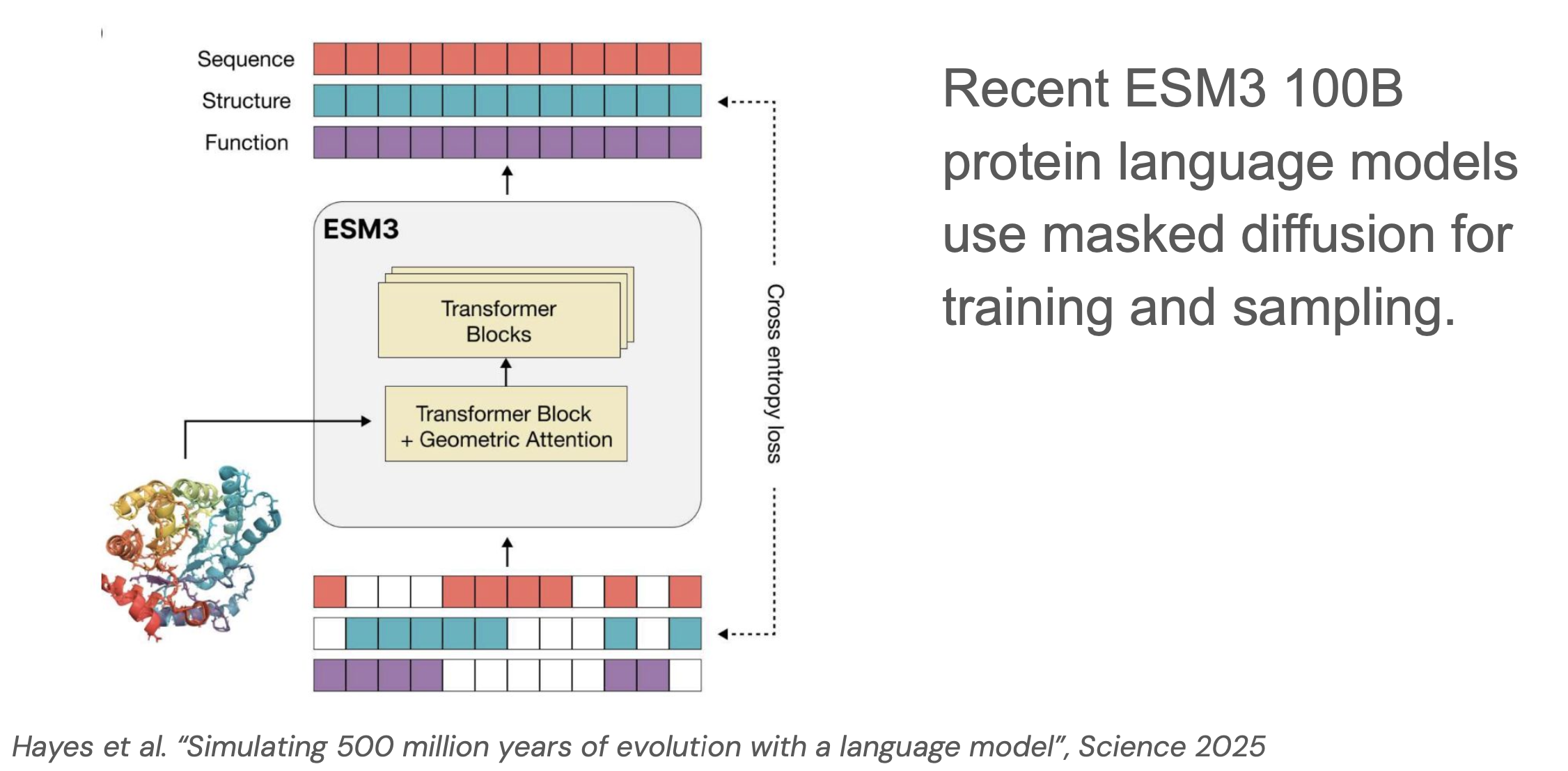
In terms of impact, the ESM models were among the first to apply large-scale sequence modeling to biological sequences. These models are widely used across proteomics for tasks such as variant effect prediction, protein folding, and protein generation.

Nucleotide Sequence Modeling

Proteins are the building blocks of life, but their activity is heavily regulated by non-coding genomic sequences that fall outside the scope of protein models like ESM3. DNA language models generalize the approach of ESM3 to both coding and non-coding genomic sequences. In a collaboration between our research group, InstaDeep, and BioNTech, we trained the Nucleotide Transformer v3 (NT-v3) family of models, which scales MDLM to billions of parameters and over a trillion tokens of DNA. These models take as input multi-track data that includes gene-expression levels alongside raw sequence. At inference time, these tracks support discrete classifier-free guidance with remasking, enabling generation of DNA sequences with target properties.

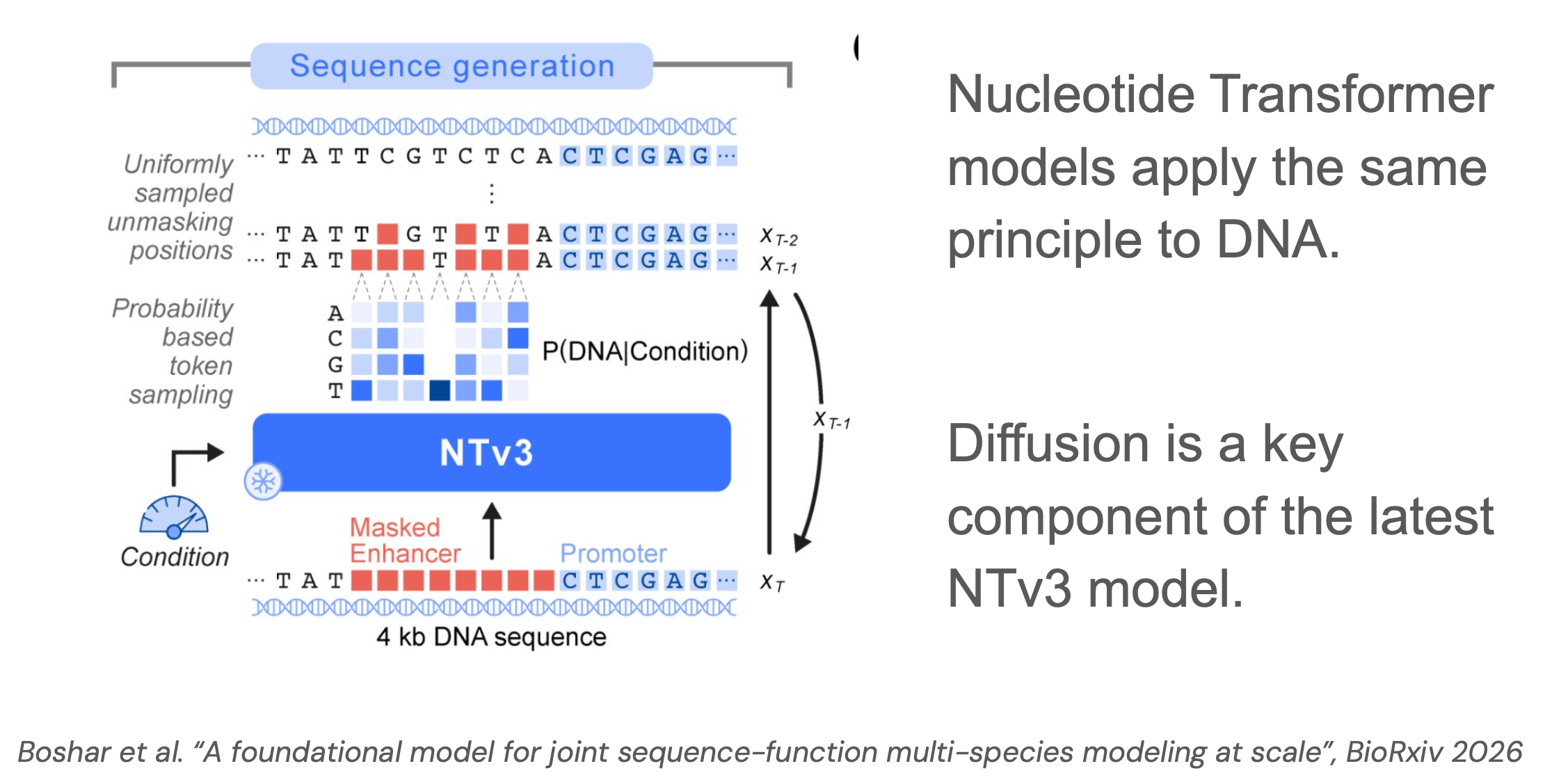
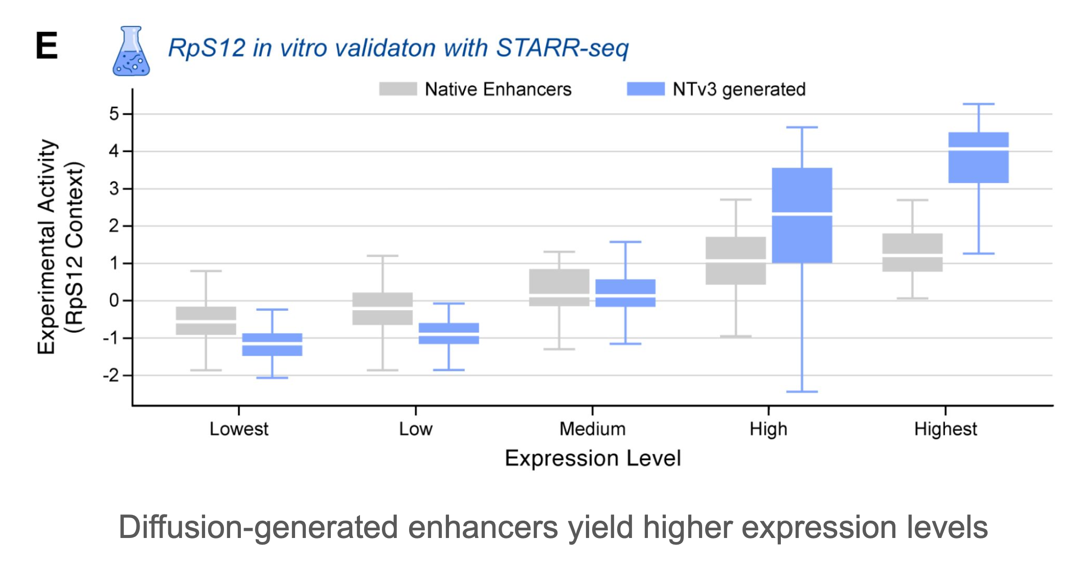
As a demonstration of the conditional generative capabilities of these models, we used NT-v3 to produce regulatory DNA sequences to enhance or repress the expression of specific genes. We generated a range of sequences by varying the guidance strength parameter in discrete CFG and we tested their capabilities in the wetlab. These generated sequences modulate gene expression better than previous baselines, and demonstrate the effectiveness of guidance.

Diffusion-Based Large Language Models

While discrete diffusion models have found early success in modeling biological sequences, the last 18 months have seen the rapid emergence of diffusion large language models.

LLaDA

LLaDA scaled MDLM to 8B parameters, emulating the LLaMA recipe, with an MDLM backbone, block diffusion at sampling time, and compatibility with remasking and post-training. It is open-weights and reports favorable scaling versus autoregressive models .

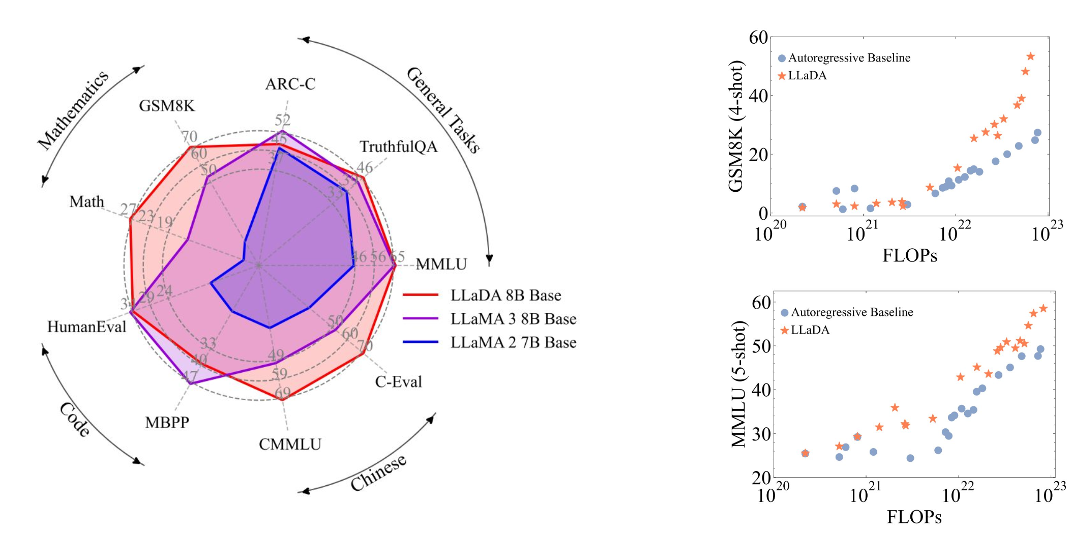
The LLaDA models are open-weights and serve as the foundation for a large body of academic research.

Mercury

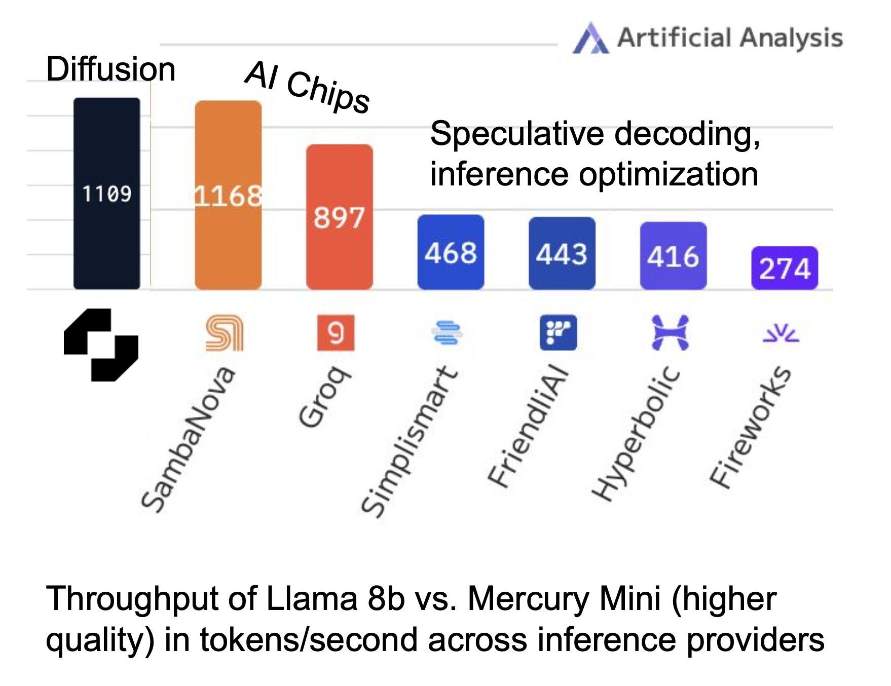
Mercury is the first commercial diffusion LLM, announced in 2025. Its differentiator is speed: leveraging parallel generation, it exceeds 1,000 tok/sec/user on standard GPUs while matching the quality of its class. Mercury 2 rivals speed-optimized frontier models (Claude Haiku, Gemini Flash-Lite/Flash) at 5–10× the speed .

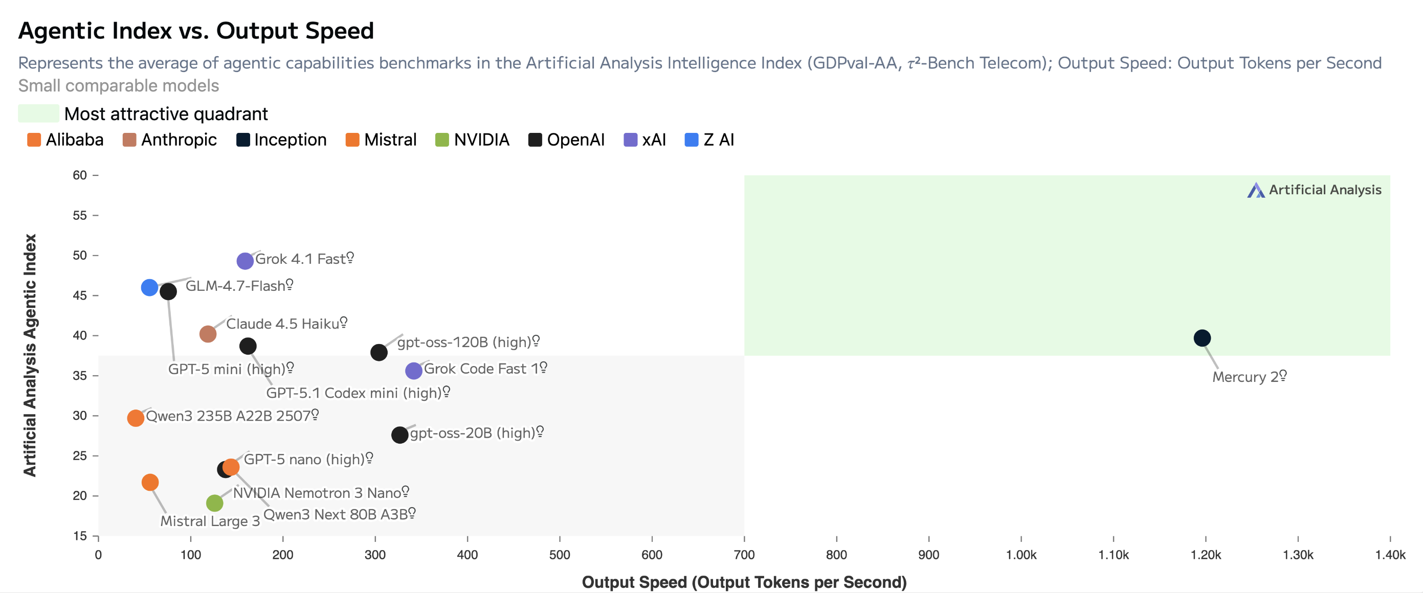
This level of speed was previously only achievable using specialized chips (e.g., Groq) purpose-built to accelerate autoregressive inference. In contrast, a diffusion model achieves comparable speeds on standard GPUs by modifying the algorithm to better fit the underlying hardware rather than the other way around.

Gemma Diffusion

Gemma Diffusion is a modern open-weights diffusion model from Google, widely supported in popular frameworks including Unsloth and Hugging Face . It combines a UDLM backbone, block diffusion for generating variable-length sequences, an encoder–decoder architecture, and accelerated sampling — shifting the generation bottleneck from memory bandwidth to compute by denoising an entire block ("canvas") of tokens in parallel on each forward pass, rather than emitting a single token at a time.

Nemotron Diffusion

Nemotron Diffusion is a family of open-weights diffusion models from NVIDIA trained with a joint autoregressive–diffusion objective, implementing MDLM and block diffusion. Recent models add an encoder-decoder architecture and scale to 35B parameters. The models report roughly 2-8× the throughput of comparable AR models while retaining up to 99% of their quality, and a single checkpoint can still fall back to plain autoregressive decoding.

Conclusion & Parting Thoughts

The field of diffusion language models has exploded over the past two years, with production-grade dLLM releases from multiple frontier labs. Diffusion offers potential advantages over autoregressive models in speed (up to 10× via parallel generation), controllability (iterative refinement for property-targeted generation), multi-modality (a single algorithmic approach across images and text), and inference-time scaling. Diffusion has not yet been scaled to the same parameters, compute, and data as autoregressive models, but experiments at up to 100B parameters show significant promise.

Is Diffusion A Path Towards More Intelligent Models? A Scaling-Law Perspective

We would like to conclude this article with an interesting question that the authors have often received when giving presentations on this work. It can be paraphrased as follows: can diffusion models eventually yield fundamental improvements over autoregressive models in terms of pure intelligence?

To answer this, we take a perspective grounded in scaling laws. The most important source of progress in model intelligence from 2019 to 2024 has surely been the scaling of pre-training in large language models. What made this scaling possible? The development of the transformer architecture, together with the wider availability of compute. But what made the transformer special? Before the transformer, the ubiquitous architecture for language models was based on RNNs. RNNs, however, never led to pre-training scaling because they did not scale — specifically, because they were fundamentally sequential algorithms that could not take full advantage of GPUs, which are highly parallel computers. It took the transformer to introduce a fully parallel training algorithm that scaled to large GPUs and unlocked the LLM revolution.

Since 2024, the gains from pre-training have been plateauing, and most of the intelligence gains in models have instead come from scaling post-training and inference-time compute. Yet both post-training and inference are bottlenecked by the ability to generate quickly, which today is done via a sequential algorithm. If inference could be made parallel, just as training was, the result could accelerate gains in intelligence as dramatic as those we saw in pre-training.

We view diffusion as the approach that could make inference fully parallel and unlock these gains. In a nutshell, diffusion may be to inference-time and post-training scaling laws what the transformer was to RNNs for pre-training scaling laws. By being able to spend more FLOPs per second, diffusion can unlock better hardware utilization, which in turn opens up our ability to scale.

It is still early to say how quickly diffusion will improve, but it suffices to say that, in our opinion, the prize is large.